. 2024 Sep 25:12:RP88608.
doi: 10.7554/eLife.88608.

A neural network model of differentiation and integration of competing memories

Affiliations

A neural network model of differentiation and integration of competing memories

Victoria J H Ritvo et al. Elife. .

Abstract

What determines when neural representations of memories move together (integrate) or apart (differentiate)? Classic supervised learning models posit that, when two stimuli predict similar outcomes, their representations should integrate. However, these models have recently been challenged by studies showing that pairing two stimuli with a shared associate can sometimes cause differentiation, depending on the parameters of the study and the brain region being examined. Here, we provide a purely unsupervised neural network model that can explain these and other related findings. The model can exhibit integration or differentiation depending on the amount of activity allowed to spread to competitors - inactive memories are not modified, connections to moderately active competitors are weakened (leading to differentiation), and connections to highly active competitors are strengthened (leading to integration). The model also makes several novel predictions - most importantly, that when differentiation occurs as a result of this unsupervised learning mechanism, it will be rapid and asymmetric, and it will give rise to anticorrelated representations in the region of the brain that is the source of the differentiation. Overall, these modeling results provide a computational explanation for a diverse set of seemingly contradictory empirical findings in the memory literature, as well as new insights into the dynamics at play during learning.

Keywords: computational modeling; fMRI; memory; neural networks; neuroscience; none; representational change; unsupervised learning.


Conflict of interest statement

VR, AN, NT, KN No competing interests declared

Figures

Figure 1.
Figure 1.. Nonmonotonic plasticity hypothesis: A has been linked to X, and B has some initial hidden-layer overlap with A.
In this network, activity is allowed to spread bidirectionally. When B is presented along with X (corresponding to a BX study trial), activity can spread downward from X to the hidden-layer units associated with A, and also — from there — to the input-layer representation of A. (A) If activity spreads strongly to the input and hidden representations of A, integration of A and B occurs due to strengthening of connections between all of the strongly activated features (green connections indicate strengthened weights; AB integration can be seen by noting the increase in the number of hidden units receiving projections from both A and B). (B) If activity spreads only moderately to the input and hidden representations of A, differentiation of A and B occurs due to weakening of connections between the moderately activated features of A and the strongly activated features of B (green and red connections indicate weights that are strengthened and weakened, respectively; AB differentiation can be seen by noting the decrease in the number of hidden units receiving strong connections from both A and B — in particular, the middle hidden unit no longer receives a strong connection from A). (C) If activity does not spread to the features of A, then neither integration nor differentiation occurs. Note that the figure illustrates the consequences of differences in competitor activation for learning, without explaining why these differences would arise. For discussion of circumstances that could lead to varying levels of competitor activation, see the simulations described in the text.
Figure 2.
Figure 2.. Basic network architecture: The characteristics of the model common to all versions we tested, with hidden- and input-layer activity for pairmate A.
Black arrows indicate projections common to all versions of the model. All projections were fully connected. Pre-wired, stronger connections between the input A unit (top row of item layer) and hidden A units (purple) are shown, and pre-wired, stronger connections between the input B unit (bottom row of item layer) and hidden B units (pink) are shown. The category unit is pre-wired to connect strongly to all hidden A and B units. Hidden A units have strong connections to other hidden A units (not shown); the same is true for hidden B units. Pre-wired, stronger connections also exist between hidden and output layers (not shown). The arrangement of these hidden-to-output connections varies for each version of the model.
Figure 3.
Figure 3.. Modeling Chanales et al., 2021.
(A) Participants in Chanales et al., 2021 learned to associate objects and faces (faces not shown here due to bioRxiv rules). The objects consisted of pairs that were identical except for their color value, and the difference between pairmate color values was systematically manipulated to adjust competition. Color memory was tested in a task where the face and colorless object were given as a cue, and participants had to use a continuous color wheel to report the color of the object. Color reports could be biased toward (+) or away from the competitor (-). (B) When color similarity was low (48°), color reports were accurate. When color similarity was raised to a moderate level (24°), repulsion occurred, such that color reports were biased systematically away from the competitor. When color similarity was raised further (6°), the repulsion effect was eliminated. (C) To model this study, we used the network structure described in Basic Network Properties, with the following modifications: This model additionally has a non-modifiable recurrent projection in the output layer, to represent the continuous nature of the color space: Each output unit was pre-wired with fixed, maximally strong weights connecting it to the seven units on either side of it (one such set of connections is shown to the output unit colored in green); background output-to-output connections (outside of these seven neighboring units) were set up to be fixed, weak, and random. The hidden layer additionally was initialized to have maximally strong (but learnable) one-to-one connections with units in the output layer, thereby ensuring that the color topography of the output layer was reflected in the hidden layer. Each of the six hidden A units were connected in an all-to-all fashion to the six pre-assigned A units in the output layer via maximally strong, pre-wired weights (purple lines). The same arrangement was made for the hidden B units (pink lines). Other connections between the output and hidden layers were initialized to lower values. In the figure, activity is shown after pairmate A is presented — the recurrent output-to-output connections let activity spread to units on either side. (D) We included six conditions in this model, corresponding to different numbers of shared units in the hidden and output layers. Three conditions are shown here. The conditions are labeled by the number of hidden/output units shared by A and B. Thus, one unit is shared by A and B in 1/6, two units are shared by A and B in 2/6, and so on. Increased overlap in the hidden and output layers is meant to reflect higher levels of color similarity in the experiment. We included overlap types from 0/6 to 5/6.
Figure 4.
Figure 4.. Model of Chanales et al., 2021 results.
(A) The distance (number of units apart) between the centers-of-mass of output activity for A and B is used to measure repulsion vs. attraction. The gray bar indicates what the color difference would be after learning if no change happens from before (gray dots) to after (black dots) learning; above the gray bar indicates repulsion and below indicates attraction. For lower levels of overlap (0/6 and 1/6), color distance remains unchanged. For a medium level of overlap (2/6), repulsion occurs, shown by the increase in the number of units between A and B. For higher levels of overlap (3/6, 4/6, and 5/6), attraction occurs, shown by the decrease in the number of units between A and B. (B) Color error (output-layer distance between the ‘guess’ and ‘correct’ centers-of-mass) is shown for each pairmate and condition (negative values indicate repulsion). When repulsion occurs (2/6), the change is driven by a distortion of pairmate 2, whereas pairmate 1 is unaffected. (C) Pairmate similarity is measured by the correlation of the hidden-layer patterns before and after learning. Here, above the gray line indicates integration and below indicates repulsion. The within-pair correlation decreases (differentiation) when competitor overlap is moderate (2/6). Within-pair correlation increases (integration) when competitor overlap is higher (3/6, 4/6, and 5/6). (D) Four hidden-layer activity patterns from a sample run in the 2/6 condition are shown: pairmate 1before, pairmate 1after, pairmate 2before, and pairmate 2after. The subscripts refer to the state of the memory before/after the learning that occurs in the color recall task; pairmate 1 designates the first of the pairmates to be presented during color recall. Brighter colors indicate the unit is more active. In this run, pairmate 1 stays in place and pairmate 2 distorts away from pairmate 1. (E) Multidimensional scaling (MDS) plots for each condition are shown, to illustrate the pattern of representational change in the hidden layer. The same four patterns as in D are plotted for each run. MDS plots were rotated, shifted, and scaled such that pairmate 1before is located at (0,0), pairmate 2before is located directly to the right of pairmate 1before, and the distance between pairmate 1before and pairmate 2before is proportional to the baseline distance between the pairmates. A jitter was applied to all points. Asymmetry in distortion can be seen in 2/6 by the movement of pairmate 2after away from pairmate 1. In conditions that integrate, most runs lead to symmetric distortion, although some runs in the 3/6 condition lead to asymmetric integration, where pairmate 2 moves toward pairmate 1before. For panels A, B, and C, error bars indicate the 95% confidence interval around the mean (computed based on 50 model runs).
Figure 5.
Figure 5.. Schematic of coactivities on Trial 1.
Generally, coactivity between pairs of units that are unique to the competitor (competitor-competitor coactivity) is less than coactivity between unique competitor units and shared units (competitor-shared coactivity), which is less than target-target, target-shared, or shared-shared coactivity. The heights of the vertical bars in the bottom row indicate activity levels for particular hidden units. The top row plots coactivity values for a subset of the pairings between units (those highlighted by the arcs in the bottom row), illustrating where they fall on the U-shaped learning function. (A) Schematic of the typical arrangement of coactivity in the hidden-hidden connections and item-hidden connections in the 2/6 condition. The competitor units do not activate strongly. As a result, the competitor-shared connections are severed because they fall in the dip of the U-shaped function; this, in turn, leads to differentiation. (B) Typical arrangement of coactivity in the higher overlap conditions, 4/6 and 5/6. Here, the competitor units are highly active. Consequently, all connection types fall on the right side of the U-shaped function, leading to integration. Specifically, all units connect to each other more strongly, leading units previously associated with either pairmate A or B to join together. (C) As competitor pop-up increases, moving from the situation depicted in panel A to panel B, intermediate levels of competitor activity can result in competitor-competitor coactivity levels falling into the dip of the U-shaped function. If enough competitor-competitor connections weaken, while competitor-shared connections strengthen, this imbalance can lead to an asymmetric form of integration where pairmate 2 moves toward pairmate 1 (see text for details). This happens in some runs of the 3/6 overlap condition.
Figure 6.
Figure 6.. Learning rate and representational change.
(A) The learning rate (LRate) parameter was adjusted and the within-pair correlation in the hidden layer was calculated for each overlap condition. In each plot, the gray horizontal bar indicates baseline similarity (prior to NMPH learning); values above the gray bar indicate integration and values below the gray bar indicate differentiation. Error bars indicate the 95% confidence interval around the mean (computed based on 50 model runs). The default LRate for simulations in this paper is 1. In the low overlap conditions (0/6 and 1/6), adjusting the LRate has no impact on representational change. In the 2/6 condition, differentiation does not occur if the LRate is lowered. In the high overlap conditions (3/6, 4/6, and 5/6), integration occurs regardless of the LRate (assuming it is set above zero). (B) For each LRate value tested, the within-pair correlation over time in the 2/6 condition is shown, where each purple line is a separate run (darker purple lines indicate many lines superimposed on top of each other). When LRate is set to 0.50 or higher, some model runs show abrupt, strong differentiation, resulting in negative within-pair correlation values; these negative values indicate that the hidden representation of one pairmate specifically excludes units that belong to the other pairmate.
Figure 7.
Figure 7.. Modeling Favila et al., 2016.
(A) Participants learned to associate individual scenes with faces (faces not shown here due to bioRxiv rules). Each scene had a pairmate (another, similar image from the same scene category, e.g., another barn), and categories were not re-used across pairs (e.g. if the stimulus set included a pair of barns, then none of the other scenes would be barns). Pairmates could be associated with the same face, different faces, or no face at all (not shown). Participants were scanned while looking at each individual scene in order to get a measure of neural representations for each scene. This panel was adapted from Figure 1 of Favila et al., 2016. (B) Neural similarity was measured by correlating scene-evoked patterns of fMRI activity. A scene pair difference score was calculated by subtracting non-pairmate similarity from pairmate similarity; this measure shows the relative representational distance of pairmates. Results for the different-face and same-face condition in the hippocampus are shown here: Linking scenes to the same face led to a negative scene pair difference score, indicating that scenes became less similar to each other than they were to non-pairmates (differentiation). This panel was adapted from Figure 2 of Favila et al., 2016. (C) To model this study, we used the same basic structure that was described in Basic Network Properties. In this model, the category layer represents the type of scene (e.g. barn, bridge, etc.), and the item layer represents an individual scene. The output layer represents the face associate. Activity shown is for pairmate A in the same-face condition. Category-to-hidden, item-to-hidden and hidden-to-hidden connections are pre-wired similarly to the 2/6 condition of our model of Chanales et al., 2021 (see Figure 2). The hidden A and B units have random, low-strength connections to all output units, but are additionally pre-wired to connect strongly to either one or two units in the output layer. In the different-face condition, hidden A and B units are pre-wired to connect to two different face units, but in the same-face condition, they are pre-wired to connect to the same face unit. (D) This model has two conditions: same face and different face. The only difference between conditions is whether the hidden A and B units connect to the same or different face unit in the output layer.
Figure 8.
Figure 8.. Model of Favila et al., 2016 results.
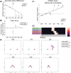
(A) Within-pair correlation between A and B hidden layer representations before and after learning. Error bars indicate the 95% confidence interval around the mean (computed based on 50 model runs). In the same-face condition, the within-pair correlation is reduced after learning, indicating differentiation. (B) Activity patterns of both pairmates in the hidden layer before and after learning for a sample “same-face” run are shown. Asymmetry in distortion can be seen in how pairmate 1’s representation is unchanged and pairmate 2 picks up additional units that did not previously belong to either item (note that there is no topography in the hidden layer in this simulation, so we would not expect the newly-acquired hidden units to fall on one side or the other of the layer). (C) MDS plots for each condition illustrate representational change in the hidden layer. The differentiation in the same-face condition is asymmetric: Pairmate 2after generally moves further away from pairmate 1 in representational space, while pairmate 1 generally does not change.
Figure 8—figure supplement 1.
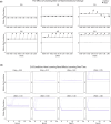
Figure 8—figure supplement 1.. Results from an alternative parameterization, where the different-face condition shows some differentiation and the same-face condition shows more differentiation.
Results from our model of Favila et al., 2016, using an alternative parameterization where the oscillation amplitude Osc for the hidden layer is set to 0.1 instead of 0.067: (A) Within-pair correlation between A and B hidden layer representations before and after learning. Error bars indicate the 95% confidence interval around the mean (computed based on 50 model runs). Compare with Figure 8A. When Osc is set to 0.1, both the different-face and same-face conditions show a reduction in pattern similarity compared to baseline, but the size of this decrease is larger in the same-face condition. This pattern of results qualitatively aligns with the actual results observed by Favila et al., 2016. (B) Plots of the within-pair correlation across learning epochs, shown separately for the different-face and same-face conditions. Each purple line is a separate run of the model (darker purple lines indicate many lines superimposed on top of each other). The plots show that individual model runs exhibit one of three discrete outcomes (integration, reflected by a within-pair correlation of 1; no change; or differentiation, reflected by a negative within-pair correlation). The differences in average levels of representational change shown in part (A) for the same-face and different-face conditions are due to differences in the frequencies-of-occurrence of these three discrete outcomes.
Figure 9.
Figure 9.. Modeling Schlichting et al., 2015.
(A) Participants in Schlichting et al., 2015 learned to link novel objects with a common associate (i.e., AX and BX). Sometimes these associates were learned in a blocked design (i.e. all AX before any BX), and sometimes they were learned in an interleaved design. The items were shown side-by-side, and participants were not explicitly told the structure of the shared items. Before and after learning, participants were scanned while observing each item alone, in order to get a measure of the neural representation of each object. This panel was adapted from Figure 1 of Schlichting et al., 2015. (B) Some brain regions (e.g. right posterior hippocampus) showed differentiation for both blocked and interleaved conditions, some regions (e.g. left mPFC) showed integration for both conditions, and other regions (e.g. right anterior hippocampus) showed integration in the blocked condition but differentiation in the interleaved condition. This panel was adapted from Figures 3, 4 and 5 of Schlichting et al., 2015. (C) To model this study, we used the network structure described in Basic Network Properties, with the following modifications: The structure of the network was similar to the same-face condition in our model of Favila et al., 2016 (see Figure 7), except we altered the connection strength from units in the hidden layer to the output unit corresponding to the shared item (item X) to simulate what would happen depending on the learning curriculum. In both conditions, the pre-wired connection linking the item B hidden units to the item X output unit is set to .7. In the interleaved condition, the connection linking the item A hidden units to the item X output unit is set to .8, to reflect some amount of initial AX learning. In the blocked condition, the connection linking the item A hidden units to the item X output unit is set a higher value (0.999), to reflect extra AX learning. (D) Illustration of the input and output patterns, which were the same for the blocked and interleaved conditions (the only difference in how we modeled the conditions was in the initial connection strengths, as described above).
Figure 10.
Figure 10.. Model of Schlichting et al., 2015 results: in this model, pairmate B is always the stimulus shown first during the competitive learning part of the simulation (after initial AX learning), so we refer to pairmate B as ‘pairmate 1’ in the figure and to pairmate A as ‘pairmate 2’.
(A) Within-pair correlation between hidden-layer A and B representations is shown before and after learning; here, the oscillation amplitude Osc was set to 0.0623. In the interleaved condition, the within-pair correlation is reduced after learning, indicating differentiation. In the blocked condition, the within-pair correlation increases, indicating integration. (B) Activity patterns of both pairmates in the hidden layer before and after learning are shown for a sample run in the interleaved condition. Asymmetry in distortion can be seen in how pairmate 2, but not pairmate 1, picks up additional units that did not previously belong to either representation. (C) MDS plots for each condition illustrate the pattern of representational change in the hidden layer. In the blocked condition, the pairmates integrate and move toward each other. This integration is mostly symmetric, but on many trials it is asymmetric: Pairmate 2 moves toward pairmate 1 rather than pairmates 1 and 2 meeting in the middle. In the interleaved condition, asymmetric differentiation occurs: Pairmate 2 moves away from pairmate 1. (D) To investigate how these results might vary across brain regions with different inhibitory dynamics, we manipulated the inhibitory oscillation amplitude to change the amount of competitor pop-up. No parameters other than the inhibitory oscillation amplitude were changed. When oscillation amplitude is reduced to 0.0525, less competitor pop-up happens, and the blocked, but not interleaved, condition leads to differentiation. When oscillation amplitude is raised to 0.09, more competitor pop-up happens, and both conditions lead to integration. For panels A and D, error bars indicate the 95% confidence intervals around the mean (computed based on 50 model runs).
Figure 10—figure supplement 1.
Figure 10—figure supplement 1.. Results from an alternative parameterization, where reducing the amplitude of inhibitory oscillations leads to differentiation in both the interleaved and blocked conditions.
Results from our model of Schlichting et al., 2015, using an alternative parameterization where the connection strength between X (in the output layer) and A (in the hidden layer) is set to 0.9 in the blocked condition (instead of 0.999). (A) Within-pair correlation between hidden-layer A and B representations is shown before and after learning; here, the oscillation amplitude Osc was set to 0.0635. In the interleaved condition, the within-pair correlation is reduced after learning, indicating differentiation. In the blocked condition, the within-pair correlation increases, indicating integration. (B) Activity patterns of both pairmates in the hidden layer before and after learning are shown for a sample run in the interleaved condition. Asymmetry in distortion can be seen in how pairmate 2, but not pairmate 1, picks up additional units that did not previously belong to either representation. (C) MDS plots for each condition illustrate the pattern of representational change in the hidden layer. In the blocked condition, the pairmates integrate and move toward each other on most (but not all) trials — a subset of the trials show differentiation. In the interleaved condition, differentiation occurs on most (but not all) trials — a subset of the trials show integration. (D) To investigate how these results might vary across brain regions with different inhibitory dynamics, we manipulated the inhibitory oscillation amplitude to change the amount of competitor pop-up. No parameters other than the inhibitory oscillation amplitude were changed. When oscillation amplitude is reduced to 0.0615, less competitor pop-up happens, and here this results in both conditions showing differentiation (compare to our original results in Figure 10D, where differentiation occurred in the blocked condition but not the interleaved condition). When oscillation amplitude is raised to 0.07, more competitor pop-up happens, and both conditions lead to integration. For panels A and D, error bars indicate the 95% confidence intervals around the mean (computed based on 100 model runs).
Figure 11.
Figure 11.. Schematic of adjusted KWTA algorithm.
Units are ranked according to the amount of inhibition that would be needed to put the unit at threshold of activity. This is proportional to excitation: The more excitation the unit receives, the more inhibition is needed to cancel out the excitation and put the unit at threshold. In the classic KWTA algorithm, inhibition is set such that only the k highest ranked units activate. We added a Target Diff parameter to potentially allow more units to activate, if units are ‘tied’ with the kth unit. If a unit below the kth unit in the rank ordering of units is within Target Diff of the kth unit, then it is considered to be ‘tied’ with the kth unit, and it is allowed to activate. In this example, the 6th, 7th, and 8th unit are tied in the ranking, because the difference is less than Target Diff. Consequently, inhibition is set such that 8 units activate.
Figure 12.
Figure 12.. U-shaped learning function.
DThr, DRev, and ThrP are X-axis coordinates. DRevMag and DMaxMag are Y-axis coordinates, and indicate the amount of peak weakening or strengthening.
Figure 13.
Figure 13.. How subtle changes to activity can affect representational change: (A) Two sample activity patterns in the hidden layer during the first trial are shown.
Units are labelled as belonging to either the target, competitor, or both (shared), and vertical bars indicate activity level (along with activity values). A moderate amount of pop-up of the competitor occurs, which should lead to differentiation if the competitor-shared connections are appropriately weakened. Although the two patterns are very similar, the bottom pattern has slightly more variable activity, which could arise if the level of random noise in the strengths of the hidden-hidden connections is higher. (B) A U-shaped function for each activity pattern is shown, with the coactivity values for a subset of the hidden-unit pairings (those highlighted by the arcs in part A) plotted along the X axis. In the top example, all competitor-competitor coactivities are lower than all competitor-shared coactivities, which are in turn lower than all target-shared and target-target coactivities. This means that it is possible to preserve all of the competitor-competitor connections while severing all of the competitor-shared connections. However, in the bottom example, there is some interlacing of the competitor-competitor coactivities and competitor-shared coactivities; this scenario makes it impossible to fully preserve all competitor-competitor connections while severing all competitor-shared connections. With the U-shaped function shown here, the pattern of activity in the bottom example will result in sparing of some of the competitor-shared connections, making it less likely that differentiation will occur.
Author response image 1.
Author response image 2.
Author response image 3.
Author response image 4.
Author response image 5.
Author response image 6.

Update of

Similar articles

Cited by

References

    1. Aisa B, Mingus B, O’Reilly R. The emergent neural modeling system. Neural Networks. 2008;21:1146–1152. doi: 10.1016/j.neunet.2008.06.016. - DOI - PubMed
    1. Amer T, Davachi L. Extra-hippocampal contributions to pattern separation. eLife. 2023;12:82250. doi: 10.7554/eLife.82250. - DOI - PMC - PubMed
    1. Artola A, Bröcher S, Singer W. Different voltage-dependent thresholds for inducing long-term depression and long-term potentiation in slices of rat visual cortex. Nature. 1990;347:69–72. doi: 10.1038/347069a0. - DOI - PubMed
    1. Barnes CA, McNaughton BL, Mizumori SJ, Leonard BW, Lin LH. Comparison of spatial and temporal characteristics of neuronal activity in sequential stages of hippocampal processing. Progress in Brain Research. 1990;83:287–300. doi: 10.1016/s0079-6123(08)61257-1. - DOI - PubMed
    1. Bear MF. Bidirectional synaptic plasticity: from theory to reality. Philosophical Transactions of the Royal Society of London. Series B, Biological Sciences. 2003;358:649–655. doi: 10.1098/rstb.2002.1255. - DOI - PMC - PubMed