Nanopore sequencing and the Shasta toolkit enable efficient de novo assembly of eleven human genomes
- PMID: 32686750
- PMCID: PMC7483855
- DOI: 10.1038/s41587-020-0503-6
Nanopore sequencing and the Shasta toolkit enable efficient de novo assembly of eleven human genomes
Abstract
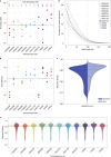
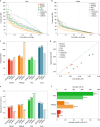
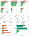
De novo assembly of a human genome using nanopore long-read sequences has been reported, but it used more than 150,000 CPU hours and weeks of wall-clock time. To enable rapid human genome assembly, we present Shasta, a de novo long-read assembler, and polishing algorithms named MarginPolish and HELEN. Using a single PromethION nanopore sequencer and our toolkit, we assembled 11 highly contiguous human genomes de novo in 9 d. We achieved roughly 63× coverage, 42-kb read N50 values and 6.5× coverage in reads >100 kb using three flow cells per sample. Shasta produced a complete haploid human genome assembly in under 6 h on a single commercial compute node. MarginPolish and HELEN polished haploid assemblies to more than 99.9% identity (Phred quality score QV = 30) with nanopore reads alone. Addition of proximity-ligation sequencing enabled near chromosome-level scaffolds for all 11 genomes. We compare our assembly performance to existing methods for diploid, haploid and trio-binned human samples and report superior accuracy and speed.
Conflict of interest statement
M.A. is a paid consultant to ONT. V.C. and S.M. are employees of ONT.
Figures


Similar articles
-
Nanopore sequencing and assembly of a human genome with ultra-long reads.Nat Biotechnol. 2018 Apr;36(4):338-345. doi: 10.1038/nbt.4060. Epub 2018 Jan 29. Nat Biotechnol. 2018. PMID: 29431738 Free PMC article.
-
Benchmarking of de novo assembly algorithms for Nanopore data reveals optimal performance of OLC approaches.BMC Genomics. 2016 Aug 22;17 Suppl 7(Suppl 7):507. doi: 10.1186/s12864-016-2895-8. BMC Genomics. 2016. PMID: 27556636 Free PMC article.
-
Are we there yet? Benchmarking low-coverage nanopore long-read sequencing for the assembling of mitochondrial genomes using the vulnerable silky shark Carcharhinus falciformis.BMC Genomics. 2022 Apr 22;23(1):320. doi: 10.1186/s12864-022-08482-z. BMC Genomics. 2022. PMID: 35459089 Free PMC article.
-
Oxford Nanopore MinION Sequencing and Genome Assembly.Genomics Proteomics Bioinformatics. 2016 Oct;14(5):265-279. doi: 10.1016/j.gpb.2016.05.004. Epub 2016 Sep 17. Genomics Proteomics Bioinformatics. 2016. PMID: 27646134 Free PMC article. Review.
-
Genome assembly in the telomere-to-telomere era.Nat Rev Genet. 2024 Sep;25(9):658-670. doi: 10.1038/s41576-024-00718-w. Epub 2024 Apr 22. Nat Rev Genet. 2024. PMID: 38649458 Review.
Cited by
-
TDFPS-Designer: an efficient toolkit for barcode design and selection in nanopore sequencing.Genome Biol. 2024 Nov 4;25(1):285. doi: 10.1186/s13059-024-03423-3. Genome Biol. 2024. PMID: 39497190
-
Optical genome mapping of structural variants in Parkinson's disease-related induced pluripotent stem cells.BMC Genomics. 2024 Oct 19;25(1):980. doi: 10.1186/s12864-024-10902-1. BMC Genomics. 2024. PMID: 39425080 Free PMC article.
-
SpLitteR: diploid genome assembly using TELL-Seq linked-reads and assembly graphs.PeerJ. 2024 Sep 27;12:e18050. doi: 10.7717/peerj.18050. eCollection 2024. PeerJ. 2024. PMID: 39351368 Free PMC article.
-
Performance of somatic structural variant calling in lung cancer using Oxford Nanopore sequencing technology.BMC Genomics. 2024 Sep 30;25(1):898. doi: 10.1186/s12864-024-10792-3. BMC Genomics. 2024. PMID: 39350042 Free PMC article.
-
Highly accurate assembly polishing with DeepPolisher.bioRxiv [Preprint]. 2024 Sep 19:2024.09.17.613505. doi: 10.1101/2024.09.17.613505. bioRxiv. 2024. PMID: 39345401 Free PMC article. Preprint.
References
-
- Poplin R, et al. A universal snp and small-indel variant caller using deep neural networks. Nat. Biotechnol. 2018;36:983–987. - PubMed
Publication types
MeSH terms
Substances
Grants and funding
- U01 HG010961/HG/NHGRI NIH HHS/United States
- U01 HL137183/HL/NHLBI NIH HHS/United States
- U41 HG010972/HG/NHGRI NIH HHS/United States
- HHMI/Howard Hughes Medical Institute/United States
- U41 HG007234/HG/NHGRI NIH HHS/United States
- T32 HG008345/HG/NHGRI NIH HHS/United States
- R01 HG010329/HG/NHGRI NIH HHS/United States
- U01 HG010971/HG/NHGRI NIH HHS/United States
- R01 HG010053/HG/NHGRI NIH HHS/United States
- R01 HG009737/HG/NHGRI NIH HHS/United States
- R01 HG010485/HG/NHGRI NIH HHS/United States
- U54 HG007990/HG/NHGRI NIH HHS/United States
- U24 HG009084/HG/NHGRI NIH HHS/United States
- R03 HG009730/HG/NHGRI NIH HHS/United States
- OT3 HL142481/HL/NHLBI NIH HHS/United States
- R44 GM134994/GM/NIGMS NIH HHS/United States
- OT2 OD026682/OD/NIH HHS/United States
- U24 HG010262/HG/NHGRI NIH HHS/United States
- R43 HG009859/HG/NHGRI NIH HHS/United States
LinkOut - more resources
Full Text Sources
Research Materials

