An actin remodeling role for Arabidopsis processing bodies revealed by their proximity interactome
- PMID: 36741000
- PMCID: PMC10152145
- DOI: 10.15252/embj.2022111885
An actin remodeling role for Arabidopsis processing bodies revealed by their proximity interactome
Abstract
Cellular condensates can comprise membrane-less ribonucleoprotein assemblies with liquid-like properties. These cellular condensates influence various biological outcomes, but their liquidity hampers their isolation and characterization. Here, we investigated the composition of the condensates known as processing bodies (PBs) in the model plant Arabidopsis thaliana through a proximity-biotinylation proteomics approach. Using in situ protein-protein interaction approaches, genetics and high-resolution dynamic imaging, we show that processing bodies comprise networks that interface with membranes. Surprisingly, the conserved component of PBs, DECAPPING PROTEIN 1 (DCP1), can localize to unique plasma membrane subdomains including cell edges and vertices. We characterized these plasma membrane interfaces and discovered a developmental module that can control cell shape. This module is regulated by DCP1, independently from its role in decapping, and the actin-nucleating SCAR-WAVE complex, whereby the DCP1-SCAR-WAVE interaction confines and enhances actin nucleation. This study reveals an unexpected function for a conserved condensate at unique membrane interfaces.
Keywords: ARP2-ARP3; LLPS; SCAR-WAVE; condensates; plasma membrane domains.
© 2023 The Authors. Published under the terms of the CC BY 4.0 license.
Conflict of interest statement
The authors declare that they have no conflict of interest.
Figures
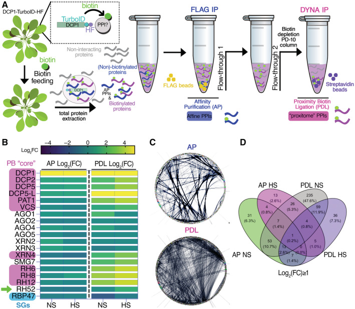
Overview of the APEAL pipeline. Upon 24 h biotin feeding and treatment (supplied with 50 μM biotin directly into leaves of 4‐week‐old plants by syringe infiltration), total proteins are extracted from infiltrated leaves. The proteome is subjected to AP‐immunocapture of the FLAG tag. In the AP step, some of the captured proteins will be biotinylated. The PDL step uses the leftover supernatant from the AP step and captures biotinylated proteins with streptavidin beads. PPI, protein–protein interactions; AP, affinity purification; PDL, proximity‐dependent biotin ligation; FLAG IP, FLAG‐beads immunoprecipitation; DYNA‐IP, streptavidin‐bead immunoprecipitation. We use the term “proxitome,” to describe the proteins captured by the PDL step of APEAL. These proteins may not physically interact with DCP1.
Heatmap showing the “core processing body (PB)” (magenta) components identified and other linked proteins. RBP47 is a stress granule marker (SGs; blue). RH52 is a new helicase identified as a PB component (green arrow). The scale on the right shows log2FC of protein abundance. Note that only the PB core components were enriched in the PDL (i.e., the proxitome, log2FC ~ 1 or above) but not in AP. Furthermore, heat stress (HS) increased the enrichment of some PB core components.
Comparison of AP/PDL interacting networks produced from APEAL. STRING density plots of pairwise interactions between proteins obtained from the AP or PDL steps (combined interactions found in non‐stress [NS]/[HS]). Note that PDL produces an overall denser interaction network (under standard parameters, the same number of proteins was selected for AP/PDL).
Venn diagram showing the proteins identified for PDL and AP in NS and HS samples (PPIs fulfilling the criterion log2FC > 1).
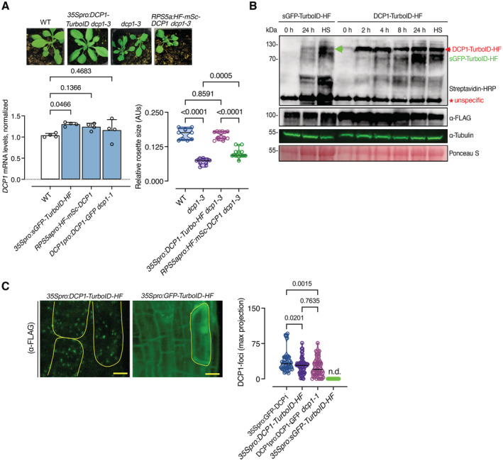
The DCP1‐TurboID‐HF construct efficiently rescues the adult dcp1‐3 mutant phenotype. Phenotypes (3‐week‐old) of adult plants expressing 35Spro:DCP1‐TurboID‐HF and RPS5apro:HF‐mScarlet‐DCP1 in the dcp1‐3 mutant background. In a semi‐controlled greenhouse setting (temperature control 22°C), the dcp1‐3 mutant showed a smaller adult stature. Lower: complementation quantification (rosette diameter), N, biological replicates = 4, n = (pooled data of 3 biological replicates) 5–7 rosettes, error bars are (mean + SD) and RT‐qPCR analyses for the quantification of DCP1 expression levels. PP2A and Actin7 were used for normalization (1‐week‐old) seedlings (N, biological replicates = 2, n (pooled data of 3 biological replicates) = 3, error bars are mean + SD). When DCP1 was driven by the RPS5a promoter (stem cell‐specific promoter), we observed partial complementation, suggesting that DCP1 is important also in non‐meristematic cells.
Immunoblot analyses of lines expressing sGFP‐TurboID‐HF or DCP1‐TurboID‐HF upon NS or HS conditions (same as used for APEAL). The immunoblots also show the accumulation of auto‐biotinylated sGFP‐TurboID‐HF or DCP1‐TurboID‐HF in a time course of biotin administration (as detected with streptavidin‐HRP, which captures biotinylated proteins). 50 μM Biotin was delivered in leaves by syringe infiltration and diffusion. Note that HS did not increase the biotinylation efficiency of DCP1‐TurboID‐HF: at 24 h, compare samples “2” with “4” in the “DynaIP”. HF, 6xhis‐3xFLAG. The red arrowhead indicates the position of DCP1‐TurboID‐HF and green for sGFP‐TurboID‐HF (N, biological replicates = 2). We used the same scheme for biotin application as determined in (Arora et al, 2020). The 2 h NS/HS corresponds to the timing after the administration of biotin for 24 h (t = 0 corresponds to 24 h biotin administration in NS conditions). The red asterisk indicates non‐specific band. α‐FLAG was used for the detection of DCP1‐TurboID‐HF and sGFP‐TurboID‐HF (similar size ~ 130 kDa). α‐Tubulin and ponceau staining were used for loading control.
Representative confocal micrographs showing that the localization of DCP1 (α‐FLAG, 5‐day‐old seedlings, root cap cells) to PBs is retained in lines expressing DCP1‐TurboID‐HF. As a control, the GFP‐TurboID‐HF line was used that does not show localization to PBs. Right: number of DCP1‐positive foci in the corresponding lines expressing DCP1 (N, biological replicates = 1, n = 32–60 cells).
- A
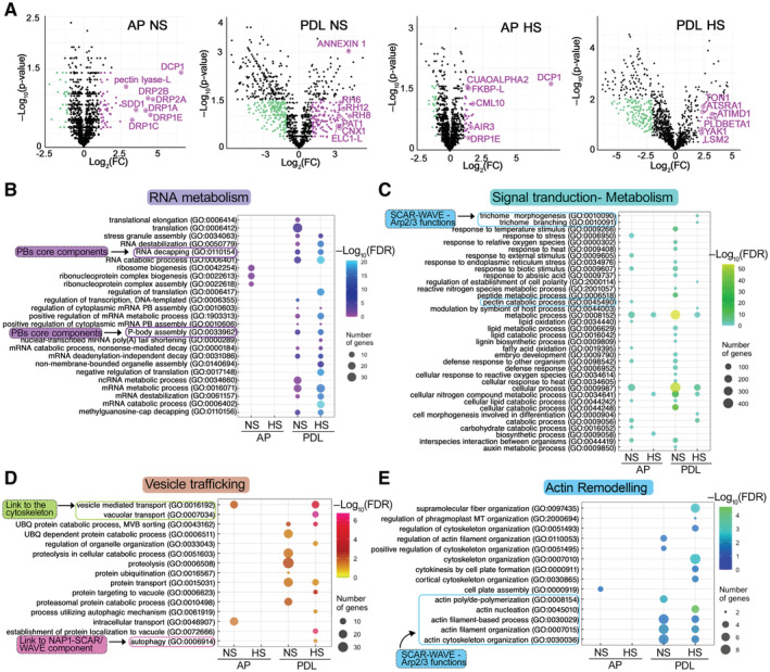
Volcano plots showing significantly enriched proteins in NS and HS conditions from the AP and PDL APEAL steps. Selected proteins are indicated in magenta and are encoded by genes that belong to the identified subnetworks described in (C) and (D). Magenta indicates enrichment in HS samples; cyan indicates depletion in HS samples.
- B–E
Gene Ontology (GO) enrichment analyses of the APEAL results, divided into four subnetworks. Note the terms related to vesicle trafficking and actin remodeling. A more detailed description is provided in Fig EV5 and in the Appendix text. Note that signal transduction proteins, metabolism‐related proteins, and vesicle trafficking proteins evade PBs during HS (Fig EV5, reduced hit number), while the opposite pattern is observed for actin and RNA metabolism subnetworks. FDR, false discovery rate. Important links described below are indicated (i.e., to the SCAR–WAVE/ARP2–ARP3 (and the component NAP1 which is part of the SCAR–WAVE and links to autophagy), cytoskeleton, PB core, and cell‐wall‐related metabolism).
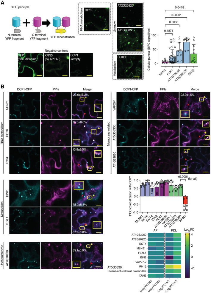
Bimolecular fluorescence complementation (BiFC) assay of the
indicated proteins. Left: the cartoon depicts the BiFC concept and YFP reconstitution caused by protein–protein interaction in vivo. When two proteins interact, the cYFP and nYFP halves are brought in proximity and produce a fluorescent signal. For protein selection, we classified the associations with DCP1, in both AP and PDL steps, according to their relative enrichment (log2FC). We selected proteins presenting moderate relative enrichment in the AP step, while having high predictability in the PDL step (log2FC > 0 in both steps). As an additional filter, we selected proteins rich in IDRs (half of the proteins from the list have high prion‐like domain (PRD) scores and high Finum [aa]/total [aa] ratios as defined through the PLAAC algorithm; Source File 8), and as such proteins would be likely to localize to condensates. We tested the association between PBs (using DCP1 as one representative component) and selected five proteins from these bins using BiFC and colocalization assays (Source File 8). These results suggested that the APEAL approach may help identify PB components or DCP1 interactors. These interactions should be further studied in Arabidopsis. BiFC efficiency was estimated from the reconstituted YFP raw signal intensity and YFP‐positive puncta per cell in maximum projections (N, biological replicates = 3, n = 4–12 cells). Lower left: representative confocal micrographs showing that YFP signal is reconstituted at cellular puncta that most likely correspond to PBs. XRN3 represents negative control (see also B), as it localizes in the nucleus. Right: number of cellular puncta per total cell volume (in maximum projection images; N, biological replicates = 3, n (pooled data of 3 biological replicates) = 20 cells, error bars are mean + SD). Scale bars: 10 μm.Colocalization of selected proteins with DCP1‐CFP‐positive puncta (35Spro:DCP1‐CFP transgene). The coding sequences of the corresponding “interactors” (PPIs; direct or indirect, defined in APEAL) were driven by the 35Spro and cloned in frame with mCherry at their 5′ end. Two‐color colocalizations were estimated by Pearson's correlation coefficients (PCC) using ultra‐fast super‐resolution microscopy combined with image deconvolution (~ 120 nm axial resolution). Numbers in “merge” indicate colocalization frequency between DCP1‐CFP and the corresponding interacting protein (N, biological replicates = 2, n = 5 cells). Yellow arrowheads indicate colocalization and red arrowheads lack of colocalization. Lower right: PCC of pixel intensities between DCP1‐CFP and the corresponding putative interacting protein (N, biological replicates = 3, n = 4–12 cells, error bars are mean + SD). We confirmed the ECT domain‐containing proteins, MLN51, FLXL1, EIN2, VAP27‐1, uncharacterized AT1G33050 (hypothetical protein), and AT5G53330/AT2G26020 (ubiquitin‐associated/translation elongation factors EF1B) as novel PB components. By applying a pre‐selection criterion of enrichment (log2FC > 0.5) for the selection of prey, we significantly increased the probability of identifying successful binary interactions between PBs (i.e., cYFP‐DCP1) and the identified proteins. All preys were confirmed as PB components, while PDL had higher interaction predictive power than the AP step irrespective of whether proteins were enriched in NS or HS. XRN3 was used as a threshold control (log2FC = −0.58, PDL/NS conditions). The heatmap shows the enrichment of these proteins in the different conditions; the scale at right shows log2FC.
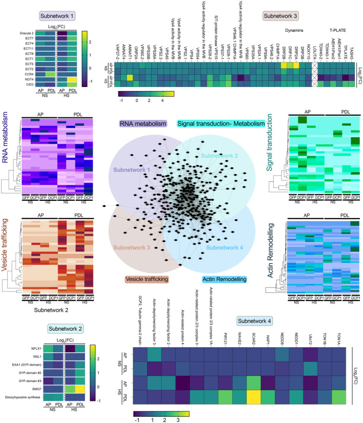
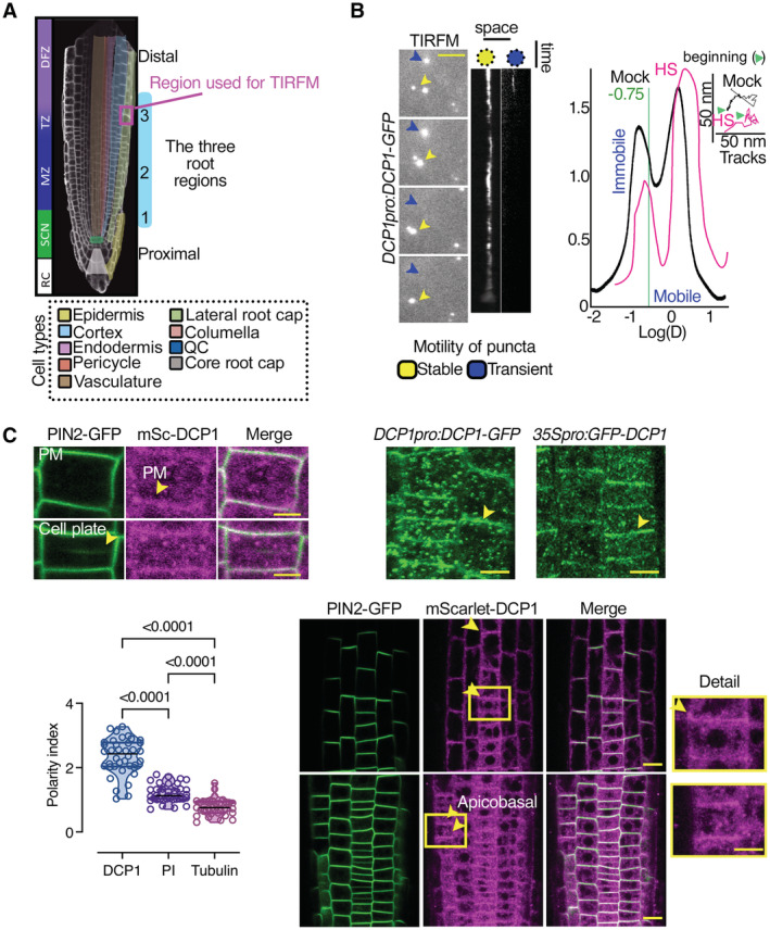
Diagram of a root showing the three developmental regions (1–3) under examination in this study: stem cell niche (SCN; region 1), meristematic zone (MZ; region 2), and transition zone (TZ)‐differentiation zone (DFZ; region 3). The different cell types are color‐coded. The region used in TIRF‐M experiments is highlighted by the dashed magenta rectangle (region 3, see also B).
Representative TIRF‐M of DCP1‐GFP (DCP1pro:DCP1‐GFP transgene) in the lateral PM of epidermal cells showing the transient attachment of DCP1‐positive puncta to the PM. Yellow arrowheads denote a PB that shows motility at the PM focal plane; blue arrowheads show a PB that transiently localizes to the PM. Scale bars: 2 μm. The corresponding kymographs are shown to the right. Right: distribution of immobile and mobile DCP1 molecules relative to the motility log(D) value of −0.75 (threshold; see Materials and Methods for details), in NS or HS conditions (D, diffusion coefficient). Inset: individual trajectories of mobile DCP1‐GFP in NS and HS conditions (500 frames, n = 120), showing a combination of directional and Brownian motion for both NS/HS. The green arrowheads denote the beginning of the NS and HS tracks for DCP1‐GFP.
Representative confocal micrographs from lines co‐expressing RPS5apro:HF‐mScarlet‐DCP1 and PIN2pro:PIN2‐GFP (epidermal cells, region 3, Scale bars: 5 μm). Bottom: polarity index of DCP1 in root meristematic cells (compared to propidium iodide (PI) and tubulin staining of root cells; N, biological replicates = 3 roots, n = 13 cells). Polarity index is calculated as the ratio of average of apical and basal VS lateral side of fluorescence signal intensity of the root epidemies cells. The arrowhead in PIN2 indicates the cell plate or PM in DCP1. Right: representative confocal micrographs showing that PM localization is independent of the promoter used (DCP1pro, 35Spro; region 2, epidermal cells, or RPS5apro on the lower right). The details from the inset show increased localization at the cell edge (discussed later). mSc, mScarlet. Scale bars: 7 μm.
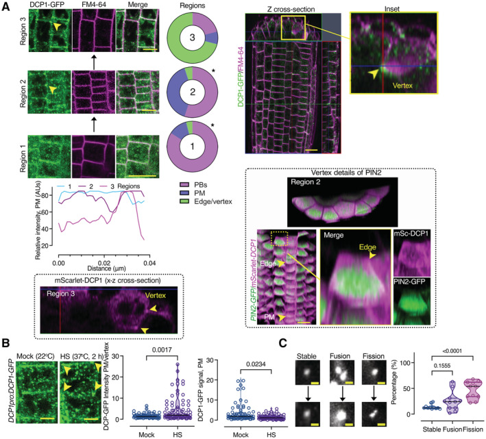
Left: Gradual edge or vertex accumulation of DCP1‐GFP in three different root regions. DCP1 signal intensity among the three different regions, at the edge/vertex (epidermis). Right: z cross‐sectional images of DCP1‐GFP (green) in the whole root compared to FM4‐64 staining (magenta, staining membranes). The circular plots indicate the average DCP1 localization (regions 1–3; N, biological replicates = 3, n = 10 cells; comparing regions 1–2 and 2–3). The 3D‐rendered images (PIN2‐GFP vs. mSCarlet‐DCP1) show the localization of mScarlet‐DCP1 at edges/vertices in two different regions (in comparison to PIN2‐GFP signal which decorated almost evenly the PM). Scale bars: 20 μm. Arrowhead denotes the edge (region 2) and the vertex (region 3) decorated by mScarlet‐DCP1 (also in the z cross‐sectional image). Note in a single cell file, how the localization from the PM changes to the edge, as indicated, along the proximodistal axis.
Representative confocal micrograph of DCP1‐GFP (DCP1pro:DCP1‐GFP, transgene) in root meristematic cells under NS/HS conditions (region 2). Scale bars, 5 μm. Note the depletion of DCP1 from the PM upon HS, but the increased edge/vertex signal (yellow arrowheads denote the vertex signal). Right: DCP1 signal intensity at the PM or edge/vertex (N, biological replicates = 3, n (pooled data of 3 biological replicates) = 18–23 PMs or edges/vertices).
Representative confocal images showing fusion (coarsening), fission, and growth of PBs (DCP1‐positive) at the PM (region 3). Right: states of PBs (dynamic: fusion and fission and non‐dynamic: stable; N, biological replicates = 2, n (pooled data of 3 biological replicates) = 6–8 PBs). As a cautionary note, the “stable” PBs may not show dynamicity in the imaging time used (~ 3–5 min) but later, may do.
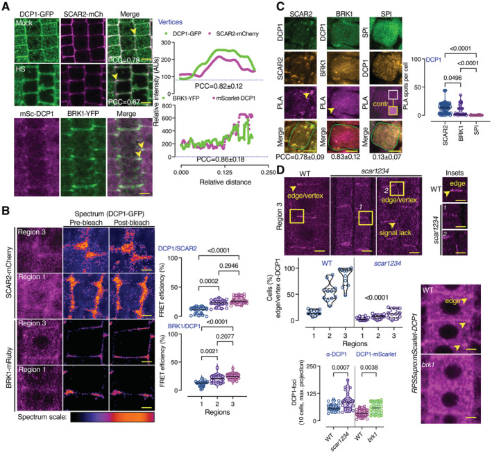
DCP1 colocalizes with the SCAR–WAVE components SCAR2 and BRK1. Representative confocal micrographs showing colocalization between DCP1 and SCAR2 or DCP1 and BRK1 (in lines coexpressing DCP1pro:DCP1‐GFP and SCAR2pro:SCAR2‐mCherry or RPS5apro:HF‐mScarlet‐DCP1 and BRK1pro:BRK1‐YFP; arrowheads indicate colocalization at cell edges or vertices) in root epidermal cells (regions 2–3). Right: relative signal intensity profiles of DCP1 or SCAR2 at vertices. Colocalization at these regions was also calculated (PCC; N, biological replicates = 2, n = 4–10 edges/vertices in regions 2–3; a slight increase was observed in HS, 0.78 in NS vs. 0.87 in HS). Scale bars: 10 μm.
Representative confocal micrographs with acceptor photobleaching‐FRET efficiency between SCAR2‐mCherry (up) or BRK1‐mRuby (down) and DCP1‐GFP (epidermal cells, regions 1 and 3). Right: normalized FRET efficiency between SCAR2 or BRK1 and DCP1, respectively, among the different developmental root regions (N, biological replicates = 2, n = 16 cells). Scale bars: 3 μm.
Representative confocal micrographs showing PLA spots produced by α‐GFP/α‐RFP in DCP1‐GFP/SCAR2‐mCherry lines and DCP1‐GFP/BRK1‐mRuby lines, α‐FLAG/α‐GFP in HF‐mScarlet‐DCP1/SPI‐YPet (SPIRRIG [SPI] is a negative control as it localizes to PBs only during salt stress and was not found in the APEAL). In the SPI PLA, a high contrast inset is presented. Right: number of PLA spots per cell (N, biological replicates = 3, n (pooled data of 3 biological replicates) = 14–33 cells). In the merged images, the cell contours are shown (light green transparent). Scale bars: 5 μm.
Representative confocal micrographs showing DCP1 localization detected by α‐DCP1 in the wild type (WT) or the scar1 scar2 scar3 scar4 (scar1234) quadruple mutant or in live‐cell imaging of mScarlet‐DCP1 (RPS5apro:HF‐mScarlet‐DCP1) in WT or brk1 mutant (bottom right; epidermal cells, region 3 for α‐DCP1 and 2 for live‐cell imaging). The arrowheads denote the lack of robust DCP1 localization in scar1234 at the edge/vertex. Small panels (insets) at right show details corresponding to the regions delineated by dashed lines, where arrowhead denotes the edge signal of DCP1 in WT; scale bars, 1 μm. Bottom: percentage of cells with proper edge/vertex localization and quantification of PB numbers (DCP1‐foci; N, biological replicates = 3, n (pooled data of 3 biological replicates) = 18–35 cells). Scale bars, 5 μm.
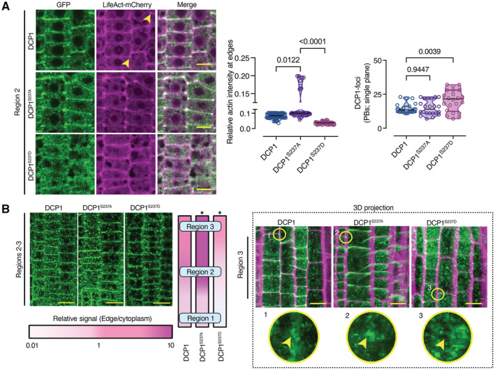
Representative confocal micrographs showing colocalization between DCP1 or two DCP1 phosphovariants with LifeAct‐mCherry in lines co‐expressing DCP1pro:DCP1‐GFP (or variants) and UBQ10pro:LifeAct‐mCherry (cell edges are indicated by yellow arrowheads). Right: relative signal intensity of actin at cell edges/vertices (normalized to the PM) in epidermal cells (N, biological replicates = 3, n = 15–30, regions 2–3). Scale bars: 7 μm.
Representative high‐resolution confocal micrographs showing the localization of DCP1‐GFP or phosphovariants (regions 2–3, epidermal cells). Left: signal at the vertex, expressed as a color‐coded edge/cytoplasmic signal ratio. Right: representative 3D projection from super‐resolution (120 nm axial, FM4‐64 counterstaining of PM) images of root meristematic cells captured from DCP1pro:DCP1‐GFP and phosphovariants (N, biological replicates = 4, n = 8). Circular insets show the differential vertex localization of DCP1 (absent in DCP1S237D‐GFP line), and arrowheads denote the vertex. Note the enhanced accumulation of DCP1S237A‐GFP at the vertex. Scale bars: 15 μm.
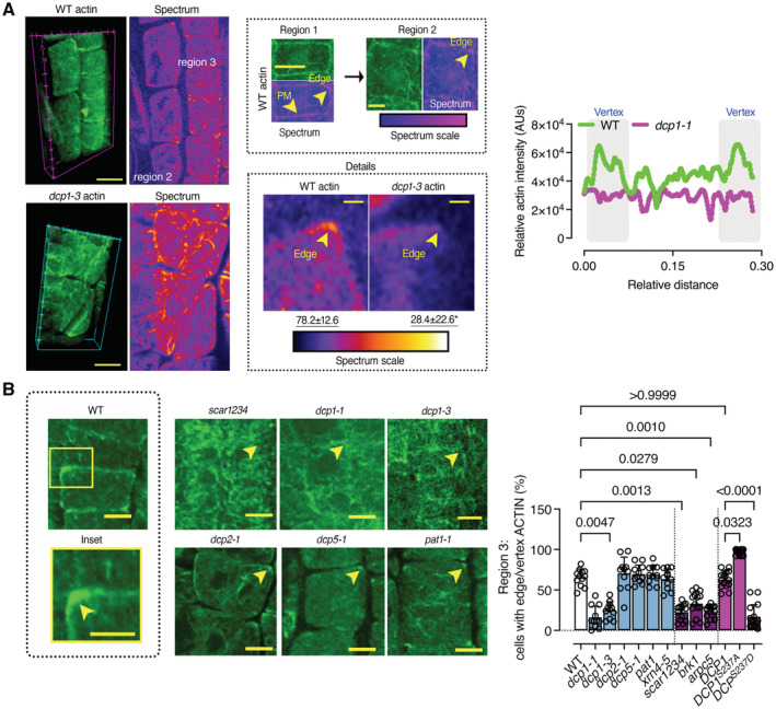
Representative confocal 3D rendering micrographs of root meristematic cells from the WT or the dcp1‐3 mutant stained with phalloidin for actin visualization (N, biological replicates = 3, n = 4). Scale bars: 5 μm (z‐scale is 4 μm). Upper middle: the “Spectrum” micrographs indicate the maximum color‐coded signal intensity (scale on the right, middle inset). Note that the signal is evenly distributed in region 1 (left upper micrograph), whereas it mostly accumulates at the edge or vertex in regions 2 and 3 (see arrowheads; images on top). Lower middle: a detail of the higher actin accumulation at edges/vertices in region 2 (compare regions 1 and 2, Scale bars: 7 μm). Insets (details, Scale bars: 2 μm) indicate the loss of vertex actin accumulation in dcp1‐3. Right: plot profile from the actin signal in the WT or dcp1‐3. The vertices are indicated.
Representative confocal micrographs showing actin localization in WT, dcp1‐1, dcp1‐3, scar1234, dcp2‐1, dcp5, and pat1 upon phalloidin staining and graph (right) indicating the percentage of cells in region 3 with an accumulation of actin at edges in various genotypes (N, biological replicates = 3, n = 7–9 roots, bars show means + s.d.). Scale bars: 7 μm.
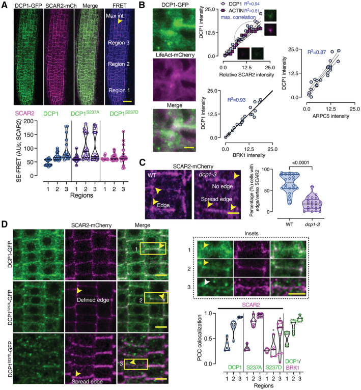
SE‐FRET efficiency between DCP1‐GFP or its phosphovariants with SCAR2‐mCherry (among the three different root regions; mainly epidermal cells). Scale bar: 50 μm. The arrowhead denotes high FRET efficiency at edges/vertices of region 3. Right: signal quantification of SE‐FRET efficiency between the indicated combinations at the epidermis of 3 regions (N, biological replicates = 6, n (pooled data of 3 biological replicates) = 10).
Actin nucleation site at an edge/vertex, as indicated by DCP1‐GFP and LifeAct‐mCherry localization. Right: correlation between DCP1 intensity, ACTIN, SCAR2, BRK1 and ARPC5 intensities (simple regression model). The R 2 values are shown, along with representative micrographs for DCP1/SCAR2 (N, biological replicates = 3, n = 6 for each point).
Representative confocal micrographs showing SCAR2‐mCherry localization in WT and dcp1‐3 mutant, respectively (root region 2, epidermal cells) and quantification of edge/vertex with SCAR2 a confined signal (N, biological replicates = 3, n = 5–8 cells).
Representative confocal micrographs showing the colocalization between DCP1‐GFP or phosphovariants and SCAR2‐mCherry in root meristematic cells (root region 2, epidermal cells). Scale bars: 10 μm. The insets show details of colocalization; the white arrowhead denotes the expansion of the SCAR2/DCP1 domain, while the yellow arrowheads the restricted edge/vertex SCAR2/DCP1 domains. Scale bars: 3 μm. The graph indicates the relative signal intensity for the indicated combinations (as Pearson's correlation coefficient; N, biological replicates = 3, n = 5 at edges/vertices: spread edges were not considered in calculations).
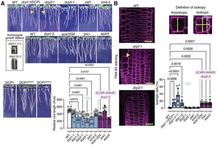
Representative images showing the phenotypes of dcp1 mutants and mutants in other PB core components or SCAR–WAVE components (5‐day‐old seedlings). The arrowheads show the growth defects of homozygous dcp1‐1 or dcp2‐1 mutants (denoted −/−; heterozygous denoted dcp1‐1/DCP1; details are also shown). Lower: graph showing relative root length (N, biological replicates = 3, n (pooled data of 3 biological replicates) = 3–4 roots, bars show means + s.d).
DCP1 regulates cell expansion anisotropy. Representative confocal micrographs showing FM4‐64 staining of the WT, dcp1‐1 and dcp2‐1 mutants (2 μM, 10 min). Scale bars, 20 μm. Right: percentage of isotropic cells per root meristem (%, epidermal cells) in each genotype (N, biological replicates = 3, n (pooled data of 3 biological replicates) = 3–5 roots, bars show means ± s.d). Examples of isotropic or anisotropic cells are shown, along with the developmental axis offset at the x‐ and y‐axes.
Similar articles
-
A proxitome-RNA-capture approach reveals that processing bodies repress coregulated hub genes.Plant Cell. 2024 Feb 26;36(3):559-584. doi: 10.1093/plcell/koad288. Plant Cell. 2024. PMID: 37971938 Free PMC article.
-
Activation of Arp2/3 complex-dependent actin polymerization by plant proteins distantly related to Scar/WAVE.Proc Natl Acad Sci U S A. 2004 Nov 16;101(46):16379-84. doi: 10.1073/pnas.0407392101. Epub 2004 Nov 8. Proc Natl Acad Sci U S A. 2004. PMID: 15534215 Free PMC article.
-
BRICK1/HSPC300 functions with SCAR and the ARP2/3 complex to regulate epidermal cell shape in Arabidopsis.Development. 2006 Mar;133(6):1091-100. doi: 10.1242/dev.02280. Epub 2006 Feb 15. Development. 2006. PMID: 16481352
-
Regulation of actin assembly by SCAR/WAVE proteins.Biochem Soc Trans. 2005 Dec;33(Pt 6):1243-6. doi: 10.1042/BST0331243. Biochem Soc Trans. 2005. PMID: 16246088 Review.
-
Nucleation, stabilization, and disassembly of branched actin networks.Trends Cell Biol. 2022 May;32(5):421-432. doi: 10.1016/j.tcb.2021.10.006. Epub 2021 Nov 23. Trends Cell Biol. 2022. PMID: 34836783 Free PMC article. Review.
Cited by
-
A proxitome-RNA-capture approach reveals that processing bodies repress coregulated hub genes.Plant Cell. 2024 Feb 26;36(3):559-584. doi: 10.1093/plcell/koad288. Plant Cell. 2024. PMID: 37971938 Free PMC article.
-
A chemical genetic screen with the EXO70 inhibitor Endosidin2 uncovers potential modulators of exocytosis in Arabidopsis.Plant Direct. 2024 Jun 14;8(6):e592. doi: 10.1002/pld3.592. eCollection 2024 Jun. Plant Direct. 2024. PMID: 38881683 Free PMC article.
-
Stress-related biomolecular condensates in plants.Plant Cell. 2023 Sep 1;35(9):3187-3204. doi: 10.1093/plcell/koad127. Plant Cell. 2023. PMID: 37162152 Free PMC article.
-
Liquid-liquid phase separation as a major mechanism of plant abiotic stress sensing and responses.Stress Biol. 2023 Dec 11;3(1):56. doi: 10.1007/s44154-023-00141-x. Stress Biol. 2023. PMID: 38078942 Free PMC article. Review.
-
A double-stranded RNA binding protein enhances drought resistance via protein phase separation in rice.Nat Commun. 2024 Mar 21;15(1):2514. doi: 10.1038/s41467-024-46754-2. Nat Commun. 2024. PMID: 38514621 Free PMC article.
References
-
- Beutel O, Maraspini R, Pombo‐Garcia K, Martin‐Lemaitre C, Honigmann A (2019) Phase separation of zonula occludens proteins drives formation of tight junctions. Cell 179: e911 - PubMed
Publication types
MeSH terms
Substances
LinkOut - more resources
Full Text Sources
Molecular Biology Databases
Research Materials
Miscellaneous