Review
. 2020 Oct 8;64(4):649-680.
doi: 10.1042/EBC20190042.

Uncovering protein structure

Affiliations
Review

Uncovering protein structure

Elliott J Stollar et al. Essays Biochem. .

Erratum in

  • Correction: Uncovering protein structure.
    Stollar EJ, Smith DP. Stollar EJ, et al. Essays Biochem. 2021 Jul 26;65(2):407. doi: 10.1042/EBC-2019-0042C_COR. Essays Biochem. 2021. PMID: 34269795 Free PMC article. No abstract available.

Abstract

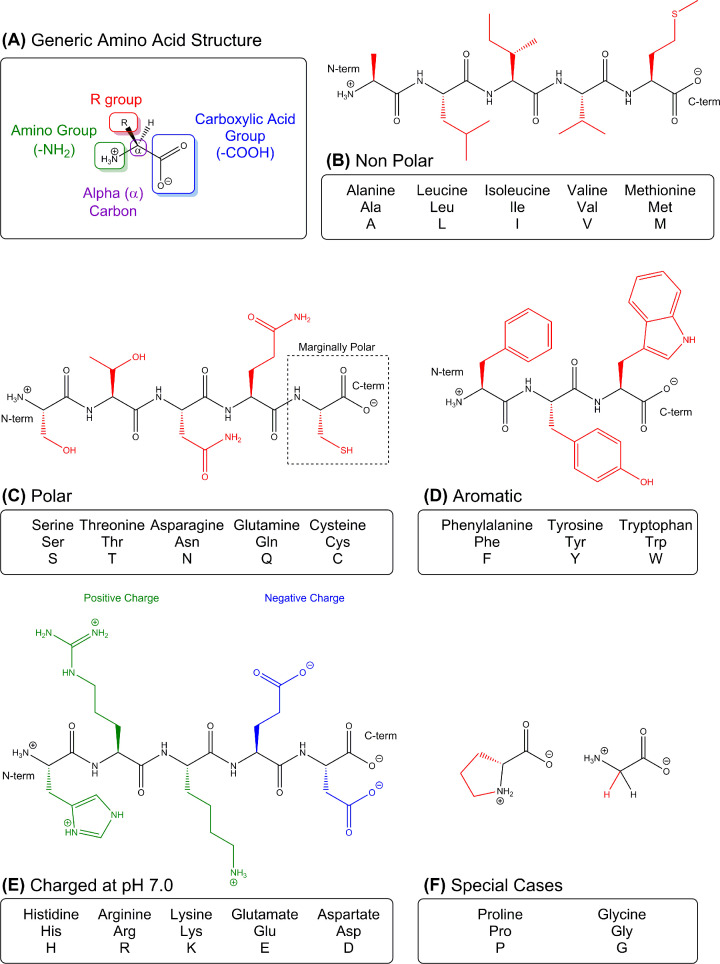
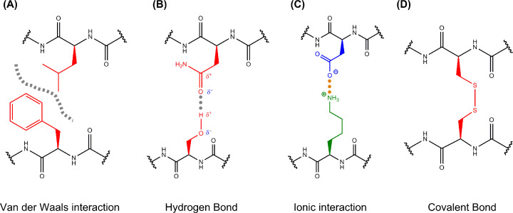
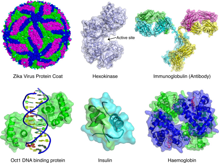
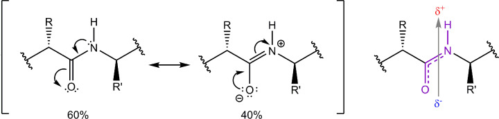
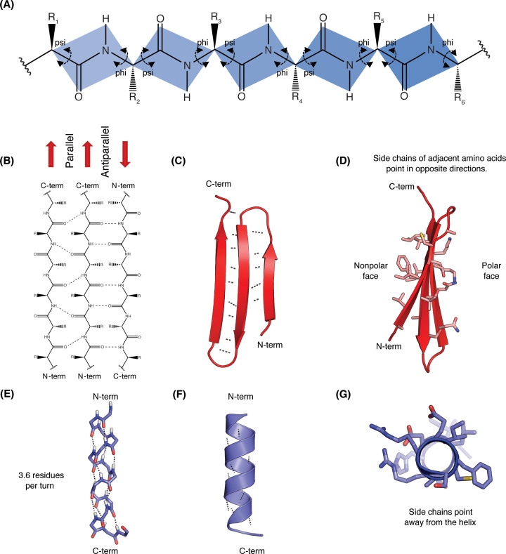
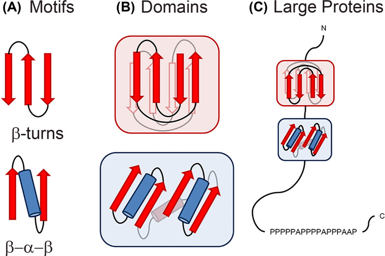
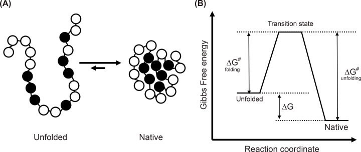
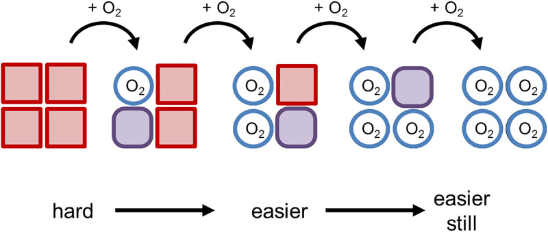
Structural biology is the study of the molecular arrangement and dynamics of biological macromolecules, particularly proteins. The resulting structures are then used to help explain how proteins function. This article gives the reader an insight into protein structure and the underlying chemistry and physics that is used to uncover protein structure. We start with the chemistry of amino acids and how they interact within, and between proteins, we also explore the four levels of protein structure and how proteins fold into discrete domains. We consider the thermodynamics of protein folding and why proteins misfold. We look at protein dynamics and how proteins can take on a range of conformations and states. In the second part of this review, we describe the variety of methods biochemists use to uncover the structure and properties of proteins that were described in the first part. Protein structural biology is a relatively new and exciting field that promises to provide atomic-level detail to more and more of the molecules that are fundamental to life processes.

Keywords: protein binding; protein chemistry; protein conformation; protein structure.


Conflict of interest statement

The authors declare that there are no competing interests associated with the manuscript.

Figures

Figure 1
Figure 1. l-Amino acids
(A) All 20 amino acids have a common structure with distinct chemical and physical properties that are determined by their R groups (side chains). Each has its own name (i.e. Alanine), three letter abbreviation (Ala) and one letter code. They are grouped according to their size, charge, polarity, and, in certain cases, by special features they impart the polypeptide backbone. Amino acids are shown as residues in short polypeptide chains with an N- and C-termini as indicated at ends. Carbon atoms do not show the letter C and are represented at bond junctions, also hydrogens attached to carbons are not shown (this representation is commonly used in organic chemistry). The polypeptide backbone is shown in black and the side chains are coloured. (B) Nonpolar residues typically have side chains that lack polar bonds and have non-polar bonds instead (i.e. they have many C–H bonds). The non-polar amino acids are hydrophobic, as they tend to cluster together to get away from water. (C) Polar amino acids are hydrophilic, meaning that their side chains interact strongly with water and each other. (D) Aromatic residues are unique in that they contain rings with alternating double bonds (tryptophan and tyrosine cannot be easily categorised as hydrophobic or hydrophilic; each has a large side chain with polar and non-polar features). (E) Charged residues are fully ionised at pH 7 and exist predominantly in their deprotonated, negatively charged form or protonated, positively charged form. In addition to side chains, the N- and C-termini of the polypeptide chain are ionised at physiological pH. (F) Glycine and Proline are shown as amino acids and are classed as special cases. Glycine has a hydrogen for a side chain and allows polypeptides to be flexible. Proline can only exist in two conformations because its side chain is directly bonded to its amino group which constrains the backbone into a narrower range of shapes.
Figure 2
Figure 2. Intermolecular interactions
Interactions between amino acid side chains help to stabilise the folded structures of proteins and allow proteins to interact with each other. These interactions can include (A) van der Waals interactions when molecules with complementary shapes approach each other. These molecules can be uncharged and only contain non-polar bonds yet at close contact, an instantaneous dipole can be induced in these non-polar bonds allowing weak electrostatic interactions between oppositely (partially) charged groups. Although an individual van der Waals force is weak, many such interactions across non-polar surfaces can allow two proteins to interact with each other. Non-polar groups can also be attracted to each other through the hydrophobic effect, which will be considered when discussing protein folding. (B) Hydrogen bonding occurs when two interacting molecules each contain dipoles (i.e. they contain polar covalent bonds), where the electrostatic attraction occurs between a partially negative N or O atom (with a lone pair of electrons) and a partially positive hydrogen atom that is covalently bound to a different N or O atom. Unlike van der Waals interactions, these bonds are not just dependent on the magnitude of the partial charges and the distance between them but also dependent on orientation of the groups involved. When the Hydrogen is linear with the covalently attached N or O and the interacting N or O (i.e. all three atoms and the lone pair of electrons appear on a line) the strength is maximal. As such, the proteins must fold and interact with other proteins using very precise geometries that satisfy this directional dependence in order to form hydrogen bonds that are strong and significant. (C) Ionic interactions (salt bridges) are attractive interactions between oppositely charged ions, since ions contain more charge than the other dipoles discussed above, they are the strongest intermolecular interaction involving charge, and (D) disulphide bonds are sulphur–sulphur covalent bonds formed by the oxidation of two cysteine residues which can be formed within a single protein chain or between two separate chains. Given these bonds are covalent, they are the strongest overall intermolecular bond, however, the bonds can be broken if a protein is exposed to reducing environments and becomes reduced.
Figure 3
Figure 3. Proteins have diverse structures and functions
Proteins are the workhorses for all living organisms and as such have an enormous range of functions that are facilitated by a range of different structures and associated dynamics. Note, the proteins shown here are not to scale and are coloured by polypeptide chain. Some proteins function to provide a structural scaffold, such as the 180 copies of envelope proteins that make up the Zika Virus outer shell which contains the RNA necessary to infect (pdb code: 5ire). Three conformations of the envelope protein are coloured differently to reveal the incredible symmetry that generates an icosahedron (20 faces) shell. Multiple copies of the monosacharide N-acetyl glucosamine are also shown (cyan). The outer shell of the virus is shown by representing the atoms in the proteins as spheres generating a surface or space-filling representation. Some proteins function as enzymes, which catalyse chemical reactions by reducing the activation barrier that must be crossed when substrates convert into products, such as Hexokinase which catalyses the first step in glycolysis (pdb code: 2yhx). This protein has a large upper (sub)domain and a smaller lower (sub)domain which creates the active site between them where catalysis occurs. When glucose binds to the active site, the domains clamp down and the mouth of the active site closes which facilitates conversion into glucose-6-phosphate using ATP. The protein is shown with a transparent surface and only the polypeptide backbone is shown inside as a cartoon representation, with thin loops connecting α-helices as spiralled tubes and β-strands as thick arrows, where the end of the arrow indicates the C-terminus. Many proteins function by binding to another protein, membrane or small molecule, to allow transport of molecules and to signal within and between cells in response to outside stimuli. For example, antibodies in the blood bind to foreign antigens (usually proteins from a foreign microorganism or virus) and elicit an immune response, which requires precise protein interactions to avoid interactions with self-proteins (pdb code: 1igt). Typically, these β-sheet rich antibodies are made up of four polypeptide chains (two long heavy chains in yellow and cyan and two shorter light chains in pink and green) that together form a stem with two flexible arms that connect to two binding sites where antigen binding occurs. The binding sites are unique for every antibody and the flexibility and dynamics of these sites allow every antibody to recognise a unique foreign molecule and attack it from multiple angles. Other examples of protein interactions include the DNA binding domain from the transcription factor Oct1 binding to DNA (pdb code: 1oct). This interaction needs to be very specific in order to only bind to the correct DNA promoter sequence so that only specific genes are turned on. The sugar–phosphate backbone of DNA is represented as a cartoon and the four DNA bases are coloured differently to highlight the unique sequence recognised by Oct1. Hormones are an important class of molecules that also rely on precise protein–protein interactions. For example, the α-helical protein insulin is a small hormone that is made of up of two chains (green and cyan) held together by disulphide bonds (pdb code: 4ins). Insulin is essential for maintaining blood glucose levels by binding to the insulin receptor found on the outside of many tissues such as liver, muscle and heart cells. Insulin binding promotes the uptake of glucose in the blood after a meal and controls many different metabolic processes by changing the activity of enzymes and transporter proteins. Finally, proteins interact specifically with small molecules to transport them across membranes or to other locations in our bodies. For example, deoxy haemoglobin is a heterotetrameric protein made up of two α subunit chains (green) and two β subunit chains (blue) that transports oxygen (pdb code: 2hhb). Each chain folds into an α-helical domain that includes a ring-like haem group (pink) containing an iron atom. Oxygen binds reversibly to these iron atoms and allows this crucial gas to be transported from the lungs in the blood to other tissues in the body. Abbreviations: ATP, adenosine triphosphate; pdb, Protein Data Bank; RNA, ribonucleic acid.
Figure 4
Figure 4. Resonance stabilisation causes the peptide bond to have double-bond character and carry a dipole
Brackets: The double-headed arrow signifies that the peptide bond is a hybrid of two states. With resonance, the nitrogen is able to donate its unhybridised lone pair of electrons to the carbonyl carbon and push electrons from the carbonyl double bond towards the oxygen, forming the oxygen anion. Right hand image: The resonance structure of the peptide bond is shown in purple. The nitrogen has a tendency to share its lone pair of electrons with the carbonyl carbon, delocalising electrons among the nitrogen, carbon and oxygen atoms. Also shown is the individual dipole moment (arrow) associated with the bond. The dashed line indicates the resonance of the peptide bond and the additional stability results in a non-rotatable peptide bond.
Figure 5
Figure 5. Protein secondary structural elements
(A) Diagram of a generic polypeptide chain. Residue side chains are denoted as R. Coloured rectangles indicate sets of six atoms that are coplanar due to the double-bond character of the peptide bond. Arrows indicate the bonds that are free to rotate with the angle of rotation about the N–Cα known as phi and about the Cα–C known as psi. Note that only peptide backbone bonds are labelled, in most cases the R group bond is free to rotate. (B) Line drawing of the chemical structure of the polypeptide backbone of three β-strands within a β-sheet. Hydrogen bonds between the main chain –CO and –NH groups are shown as dotted lines. Parallel sheets contain β-strands that run in the same direction, whereas antiparallel sheets contain β-strands that run in the opposite direction to its neighbour. (C) Cartoon representation (also known as a ribbon diagram) of an antiparallel β-sheet region from a larger protein. In this example, three β-strands are connected by a short loops. Arrows representing β-strands point towards the C-terminus by convention. The hydrogen bonds holding the sheets together are shown as dotted lines. (D) Side view of the same β-sheet showing the individual residue sidechains. The atoms are coloured with carbon in pink, sulphur in yellow, oxygen in red and nitrogen in blue. Note the residues on the non-polar side are mainly constructed from non-polar carbon containing residues whereas the residues on the polar side have oxygen and nitrogen atoms and are a mixture of ionic and polar sidechains. Each strand has a slight twist that can be seen in the image. (E) Stick representation of an α-helix with the sequence NH2–SGEFARICRDLSHIG–COOH. Hydrogen bonds between backbone atoms are indicated with dashed lines. The atoms are coloured with carbon in light blue, sulphur in yellow, oxygen in red and nitrogen in blue. Note the peptide bonds in an α-helix all point in the same direction and are bonded to a residue four places along the chain. (F) Cartoon representation of the same α-helix as seen in larger protein structures. (G) Rotated view of the α-helix, side chains radiate outwards, away from the centre of the helix.
Figure 6
Figure 6. Motifs, Domains and Full-length proteins
(A) Secondary structure often packs into motifs. These motifs are stable easily folded arrangements but cannot exist independently. (B) A protein domain is a conserved part of a given full-length protein sequence with a defined tertiary structure that can evolve, function and exist independently of the rest of the protein chain. Each domain forms a compact 3D structure and often can be independently stable and folded usually with a distinct function. (C) Large proteins are usually made up of several independently folded domains. The protein is represented by a straight line from the N- to C-termini with any protein domains it contains represented in boxes. The amino acid sequence is highlighted at the C-terminus and due to its low complexity of just proline (P) and alanine (A) is predicted to be disordered.
Figure 7
Figure 7. Two state folding of a small protein
(A) Hydrophobic collapse. In the compact fold (to the right), the hydrophobic amino acids (shown as black spheres) collapse towards the centre to become shielded from aqueous environment. (B) The classical view of protein folding. Diagram represents the free energy of the native and denatured ensembles of a protein under conditions where the native state is favoured as the native state has a lower free energy than the unfolded state. The free energy difference between these states (ΔG) is a measure of the stability of the protein. The transition state ensemble is a population of short-lived and partially folded conformations that cannot be directly observed in experiments but must be passed through to fold and defines the activation barrier for folding (ΔG# folding) and unfolding (ΔG# unfolding).
Figure 8
Figure 8. Cross-β structure of amyloid material
NMR atomic-resolution structure of an amyloid triplet fibril (right) fitted into a cryo-EM reconstruction (centre). The background image of the fibril (left) was taken using Transmision Electron Microscopy (scale bar, 50 nm). The constituent β-sheets are shown in a ribbon representation in blue; oxygen, carbon and nitrogen atoms are shown in red, grey and blue, respectively. Note that in a cross-β struture β-strands are stacked one on top of the other. Image adapted with permision from Fitzpatrick, Debelouchina, Bayro, Clare, Caporini, Bajaj, Jaroniec, Wang, Ladizhansky and Müller (2013) Atomic structure and hierarchical assembly of a cross-β amyloid fibril. Proc. Natl. Acad. Sci. U.S.A. 110, 5468–5473. Abbreviations: cryo-EM, cryogenic electron microscopy; NMR, nuclear magnetic resonance.
Figure 9
Figure 9. Positive allostery in haemoglobin
This diagram illustrates the ‘sequential’ model of cooperativity, which suggests that oxygen binding to one subunit of haemoglobin starts a sequence of conformational changes in the other haemoglobin subunits, which increase their affinity for oxygen, and that this happens in a sequence. The binding of oxygen (blue circle) in one subunit causes a structural change in a neighbouring subunit (purple) that makes them more able to bind another oxygen molecule.
Figure 10
Figure 10. Feedback inhibition in metabolic pathways
The production of the metabolite E in this four-step metabolic pathway allows it to bind to the first enzyme in the pathway to turn it off, thus regulating the amount of E in the cell. When levels of E drop, the pathway will be turned back on again as the first enzyme is no longer inhibited. Frequently this feedback inhibition is caused by negative allostery that involves a change in the conformation of the active site by another molecule binding elsewhere on the enzyme.
Figure 11
Figure 11. Cartoon of the coupled folding and binding
PUMA is an intrinsically disordered protein (green) that folds on binding to the folded MCL-1 protein (white). Before binding, PUMA is modelled as an ensemble of rapidly interconverting unfolded states.
Figures B1 and B2
Figures B1 and B2. Property of light and constructive interference
(B1) A wave of light can be described by two periodic functions representing the electric and magnetic fields that are perpendicular to each other, where their amplitude changes along the x-axis. If you draw a beam of light in the form of a wave, the distance between two crests is called the wavelength. The frequency that the waves repeat themselves determines their wavelengths. For most of our text, we only show the electric component. (B2) When light waves are in phase (start at the same position within the periodic function), light interferes constructively and they add together to make a bigger wave (top panel). Light interferes destructively annihilating each other when waves are out of phase, for example when the peak of one wave is aligned with the trough of another (bottom panel).
Figure 12
Figure 12. CD spectroscopy
Light waves can travel at any angle and through the use of a special polarising lens, light can be selected for a single plane i.e. in a vertical (represented in red) or horizontal (represented in green) plane. (A) When horizontally and vertically polarised light are combined in phase the resulting plane polarised light wave oscillates back and forth at 45 degrees (represented in blue). (B) Circularly polarised light consists of two perpendicular plane waves of equal amplitude and ¼ of a wavelength difference in phase. At a single point in space, the circularly polarised light will trace out a circle over one period of the wave shown here as a spiral. Depending on the rotation direction, it is called left-handed (LCP) or right-handed (RCP) circularly polarised light. (C) A chiral molecule such as a protein (indicated as red box) will absorb LCP and RCP as indicated by the size of each spiral to the right of the red box. CD instrument allows the absorption of LCP and RCP circularly polarised light to be measured. (D) LCP and RCP are represented as vectors on the detector. When both LCP and RCP are absorbed the same amount (left), their combination leads to a linear (blue) vector that oscillates up and down. However, when different absorption of the LCP and RCP occurs (in this case RCP has been absorbed by the protein leading to decreased amplitude) their combination leads to elliptically polarised light. This happens as when the short vector from RCP is combined with the longer vector of LCP, the resultant rotating (blue) vector now describes an ellipse. The angle made by the big axis of the ellipse with respect to the original polarisation plane is measured in degrees (θ). Only the electric components of light waves are shown for clarity (the magnetic component is always perpendicular to the electric component).
Figure 13
Figure 13. Characteristic CD spectra
CD spectroscopy can be used to estimate the secondary structural content of a protein. Each secondary structural type has a characteristic spectrum. α-helical proteins like Insulin (blue) have a double hump spectrum with peaks at negative bands at 222 and 208 nm and a positive band at 193 nm. Proteins with well-defined antiparallel β-sheets like Immunoglobulins (red) have negative bands at 218 nm and positive bands at 195 nm. Disordered proteins such as the micro-exon gene 14 (green) have very low signal above 210 nm and negative bands near 195 nm.
Figure 14
Figure 14. The X-ray crystallography set up
Protein crystals are made up of a repeating array of unit cells that contain one or more copies of a protein. When these crystals are exposed to X-rays, the light changes its path and those diffracted X-rays that undergo constructive interference are measured on a detector and are called reflections. Experiments are repeated for multiple orientations of the crystal and all measured reflections are combined to create a full set of data to be analysed by a computer to generate a protein structure.
Figure B3
Figure B3. Bragg’s Law
Two in-phase waves R1 and R2 (shown as straight lines instead of oscillating waves) are scattered by an angle θ, relative to the periodic array (red dots). If the additional distance travelled by R2 (i.e. two times the distance BC) is a whole number of wavelengths, n, then the waves will remain in phase and give constructive interference. If the extra distance travelled by R2 to cover 2BC was a fraction of a wavelength (for example 0.5 of a wavelength), then the peaks and troughs of R2 would be shifted relative to R1 and the waves would cancel out through destructive interference. For R2, a line is shown going through point B to indicate that the waves diffract with an angle of 2θ with respect to the original X-ray beam.
Figure 15
Figure 15. Fourier Transformation
The Fourier mathematical operation sums the contributions of several simple functions with different frequencies, amplitudes and phases (on left) to make a complicated function (on right). Simple functions could be used to describe each reflection in a diffraction pattern or each electron position in a protein crystal. Complicated functions generated after transforming a set of reflections or set of electrons could be a complete electron density map or a complete diffraction pattern respectively. To get sufficient signal from a crystal, Bragg’s law must be obeyed, which is only satisfied for certain diffraction events that limits the number of reflections to be Fourier transformed after a diffraction experiment. In this example, all waves are in phase but most waves representing reflections are usually out of phase with each other, meaning they would not all start at the same point on the curve and their phases would need to be estimated in order to solve the phase problem. NMR also uses the Fourier transformation to convert a complicated FID generated from multiple atoms into a series of simple functions with different frequencies and amplitudes.
Figure 16
Figure 16. An electron density map
Electron density map can be calculated using the information from the intensities of experimental reflections combined with the best possible phases. A model (shown as sticks and balls) can be built into this electron density (sticks). Post-refinement electron density is from human synaptotagmin 1 C2B domain.
Figure 17
Figure 17. How bulk magnetisation is generated and manipulated for multiple copies of the same atom
A given atom in a protein is represented as many vectors (with different directions) as there will be many copies in the sample (bottom panel). The individual vectors average (or sum) to generate a bulk magnetisation vector (thick black line) with properties that represent all of these identical atoms (top panel). Before an external magnetic field (B0) is applied, individual vectors point in all directions and no bulk magnetisation vector is present (left). However, after a B0 field is applied (grey arrow in bottom panel) the sample generates a net magnetisation along the magnetic field direction (the z-axis) which can be represented by a bulk magnetisation vector (thick black arrow in top panel). When a short RF-Pulse (along the x-axis) has been applied, the bulk magnetisation is nudged into the x–y plane and immediately afterwards starts to rotate about the z-axis in a corkscrew motion at its Larmor frequency (chemical shift) as it returns back to its equilibrium position. The x-component of the rotating bulk magnetisation following the pulse is measured by the spectrometer’s coil as a decaying oscillating electric field called an FID. The RF-pulse is effective as it generates a short-lived oscillating B1 magnetic field in the coil, along the x-axis, which is at the same Larmor frequency of the nuclei under study, allowing it to rotate magnetisation toward the x–y plane. This is similar to effectively pushing a child on a swing, one constant push (constant B1) is not as effective as pushing with the natural frequency of the swing (oscillating B1). This vector model only really applies to spins that are not ‘coupled’ to another spin and for a deeper understanding of NMR, we would need to consider the subatomic quantum realm, where conventional/familiar, classical physics, does not apply and is beyond the scope of this text.
Figure 18
Figure 18. An 1H FID for a protein and its Fourier Transform
The FID on the left is the sum of FIDs for each different Hydrogen nucleus in the protein. Fourier transformation of this FID creates a set of component frequencies (seen as a peak for each individual FID). Conversion of Larmor frequency (Hz) into chemical shift (ppm) as seen in the 1D 1H NMR spectrum of a protein allows for values to be independent of the magnet strength used. Each peak represents the hydrogen atoms connected to different carbons or nitrogens in the protein. The chemical shifts are different because the 1H nuclei all experience slightly different magnetic environments based on their chemical group and position in the protein and thus their bulk magnetisation vectors rotate at slightly different frequencies. Hydrogens found in common chemical groups (in amides, aromatics, aliphatics, methyl etc.) are indicated above the spectrum. The well-dispersed peaks between 6 and 10 ppm in the backbone amide region indicate that the protein is well folded. It is common to make a higher dimensional spectrum such as the 2D spectrum that plots the chemical shift values for pairs of atoms connected by a covalent bond to better resolve the overlapping signals. Abbreviation: 2D, two dimensional.
Figure 19
Figure 19. 1H 15N-HSQC of a small protein domain
Each numbered peak in this 2D spectrum represents an amino acid in a simple protein domain through its backbone (or sidechain) amide group. An amide group has one nitrogen and one hydrogen and given each amino acid is in a slightly different chemical environment based on how the protein has folded and which sidechain it contains, the chemical shift values for each N and H pair are different for each amino acid. This creates a unique “fingerprint” identification for every protein.
Figure 20
Figure 20. Cryo-EM process
Image processing outline illustrated with data from the small pore-forming toxin lysenin. To capture the initial images, protein samples are transferred onto a copper mesh grid coated with a perforated carbon film. The sample is then flash frozen in ethane at −190°C, causing the water to vitrify and capturing the proteins in random orientations within the holes of the carbon film. A beam of electrons is then use to capture a faint trace image of the protein. The computer determines what is protein and what is background. Similar images of the protein in the same orientation are placed into the groups. Using thousands of similar images of the protein, the computer generates a high-resolution 2D image by averaging all the faint images. A 3D image is then calculated by working out how the 2D images relate to each other producing an electron density map from which the structure is then determined. Image from Savva (2019) A beginner’s guide to cryogenic electron microscopy. Biochemist41, 46–52.

Similar articles

Cited by

References

    1. Doucleff M., Hatcher-Skeers M. and Crane N.J. (2011) Pocket Guide to Biomolecular NMR, Springer
    1. Zoran P., David B., Firas K., Seth C., Jens M., Scott H. (2008) Fold your own protein, https://fold.it/
    1. Jonsson A.L., Roberts M.A.J., Kiappes J.L. and Scott K.A. (2017) Essential chemistry for biochemists. Essays Biochem. 61, 401–427 10.1042/EBC20160094 - DOI - PMC - PubMed
    1. Johnson M.P. (2016) Photosynthesis. Essays Biochem. 60, 255–273 10.1042/EBC20160016 - DOI - PMC - PubMed
    1. David S.G., Alexander R., Maria V., Rob L. (2020) Molecular machinery: a tour of the Protein Data Bank. https://cdn.rcsb.org/pdb101/molecular-machinery/