. 2014 Mar;111(5):1132-49.
doi: 10.1152/jn.00785.2013. Epub 2013 Dec 18.

Large-scale, high-density (up to 512 channels) recording of local circuits in behaving animals

Affiliations

Large-scale, high-density (up to 512 channels) recording of local circuits in behaving animals

Antal Berényi et al. J Neurophysiol. 2014 Mar.

Abstract

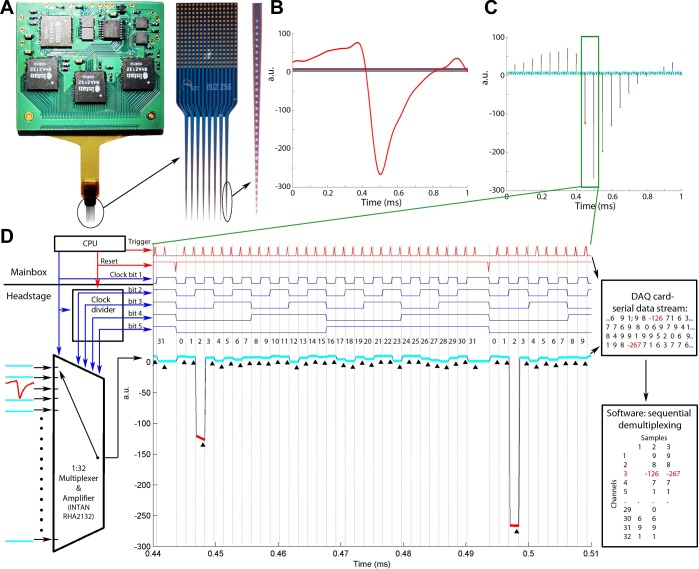
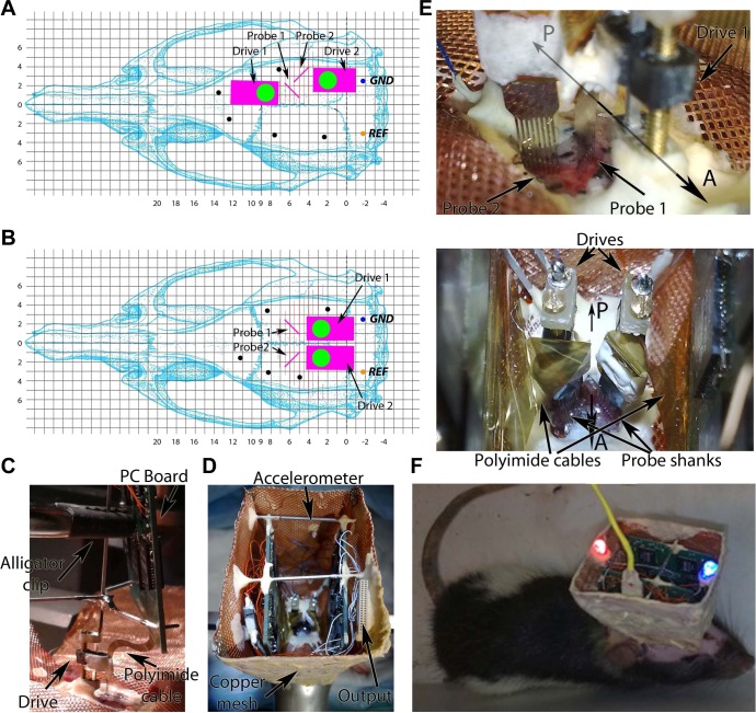
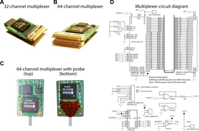
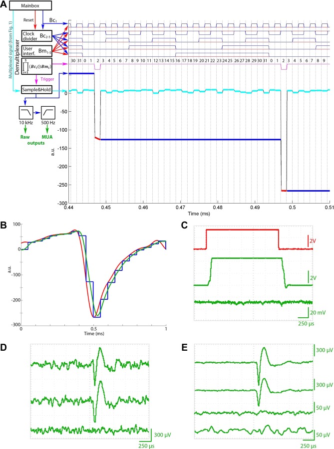
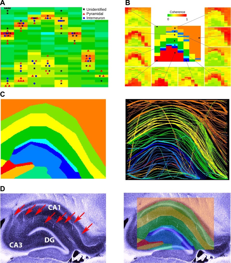
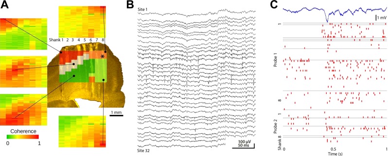
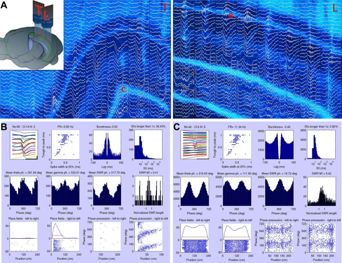
Monitoring representative fractions of neurons from multiple brain circuits in behaving animals is necessary for understanding neuronal computation. Here, we describe a system that allows high-channel-count recordings from a small volume of neuronal tissue using a lightweight signal multiplexing headstage that permits free behavior of small rodents. The system integrates multishank, high-density recording silicon probes, ultraflexible interconnects, and a miniaturized microdrive. These improvements allowed for simultaneous recordings of local field potentials and unit activity from hundreds of sites without confining free movements of the animal. The advantages of large-scale recordings are illustrated by determining the electroanatomic boundaries of layers and regions in the hippocampus and neocortex and constructing a circuit diagram of functional connections among neurons in real anatomic space. These methods will allow the investigation of circuit operations and behavior-dependent interregional interactions for testing hypotheses of neural networks and brain function.

Keywords: behaving rats and mice; local field potential; monosynaptic connections; unit firing.


Figures

Fig. 1.
Fig. 1.
System overview. A: high-channel-count (256 sites) silicon probe connected to a printed circuit board via a flexible polyimide ribbon cable. The printed circuit board contains 8 separate 32-channel signal multiplexers (4 on each side) and accessory circuit elements. B: a simulated headstage input signal illustrating a spike waveform on 1 of the 32 channels and various levels of direct current (DC) on the remaining 31 channels (1 ms). a.u., Arbitrary units. C: time-shared multiplexed signal transmitting the 32 channels shown in B. D: circuit schematics and working principle of the multiplexer and a zoomed segment of the time epoch shown by rectangle in C. The multiplexer chip receives the input signals and is driven by both the clock signal of the main microcontroller and the complementary clock bits generated by the clock divider. The horizontal line separates circuits contained in the headstage and the main box. Middle part: zoomed segment of the multiplexed signal shown in B. The reset line resets the clock bits to “00000” after every 32 steps to ensure the proper channel order. The trigger signal is timed to sample the “tail” of each transmitted signal snippet (marked by black triangles). The 2 large steps (red) correspond to the 2 digital samples at the trough of the spike waveform on input channel 3. Right part: numerical representation of the analog-to-digital (A/D)-converted multiplexed line (readout from the A/D card) and its demultiplexed form after the software reconstruction of the digitized samples. CPU, central processing unit.
Fig. 2.
Fig. 2.
Surgery details of probe implantation. A and B: skull coordinates for implantation of 2 256-site probes into the same (A) or 2 hemispheres (B). The orientation of the probe shanks is indicated by pink lines next to the probe drives. Black dots: watch screws. GND, ground; REF, reference electrode. C: during probe implantation, the probe and the printed circuit (PC) board are rigidly connected by brass rods, and the assembly is held by an alligator clip. The probe is fixed to the drive and connected to the PC board by a flexible polyimide cable. D: the headstage after implantation. The output connector, accelerometer, and copper wire mesh shield are marked by arrows. E: details of the probe shanks after they penetrated the brain. A, anterior; P, posterior direction. Bottom: top view of the implanted drives. F: rat equipped with 2 256-site probes during maze exploration connected to the equipment via an ultraflexible cable (yellow).
Fig. 3.
Fig. 3.
Headstage multiplexers. A and B: 32- and 64-channel multiplexers with high-density Omnetics connectors. C: 64-site probe bonded to a 64-channel multiplexer. D: circuit schematics representing the electrical components and wiring scheme of the 32-channel multiplexer. Top: wiring diagram of the Intan RHA-2132 multiplexer chips and the high-density Omnetics connector for electrode interfacing. The cutoff frequencies of the low- and high-pass filters are set with the 3 resistors on the left. Bottom: supplementary electronics to provide clock bits and buffer the signal. Top row, left to right: 9-pin Omnetics connector interfaces with the main box; high-speed, dual-buffer operational amplifier. Bottom row: synchronous clock divider chip; external light-emitting diode (LED) power port for position tracking; clock inverter chip with Schmitt trigger; decoupling capacitor.
Fig. 4.
Fig. 4.
Demultiplexer circuit. A: working principle of the real-time demultiplexer. The clock signal from the main box (Fig. 1) is successively halved 4 times to produce 4 subsequent clock bits (blue trace, Bc1..5). A clock-bit-mask pattern set by the user interface (interf.; Bm1..5, red traces) is pairwise-compared (XNORed) with the clock bits, and the results are logically ANDed. The output of this logical operation is the trigger (pink trace), which switches the sample-and-hold circuit so that when the clock bits match the preset mask the circuit works as a relay (1/32nd of the running cycle); otherwise, it holds the last sampled voltage (31/32nd of the running cycle). The output of the sample-and-hold circuit is shown as red and blue lines for the sampling and holding periods, respectively. The example demultiplexes channel 2. The demultiplexed signal trace is low-pass filtered to remove the step functions and optionally high-pass filtered at 500 Hz to separate unit firing from the local field potential (LFP). MUA, multiunit activity. B: temporal delay of the demultiplexing process. Red trace: original input waveform; blue trace: output of the sample-and-hold circuit; green trace: low-pass filtered signal at the output of the demultiplexer. C: signal transmission characteristics of the demultiplexer for a large-amplitude step function. Red trace: original input signal; upper green trace: demultiplexed waveform; lower green trace: demultiplexed signal on an adjacent channel in the multiplexed sequence. Note the different amplitude scales for the traces. D: single trace examples of a demultiplexed unit. The top 2 traces represent 2 waveforms representing 2 distinct projections of the spike onto 2 adjacent recording sites of the probe. The bottom trace shows the signal recorded on neighboring channel in the multiplexed stream. E: spike-triggered average waveforms of the neuron shown on D. Note the lack of cross talk in both the temporal (incomplete signal level settling during multiplexing or demultiplexing, 3rd trace) and spatial (cross talk across leads, 4th trace) domain.
Fig. 5.
Fig. 5.
Electroanatomy of the hippocampus. A: distribution of high-frequency power (300 ± 10 Hz) on each of the 256 sites of the silicon probe. The 32 × 8 color matrix is a representation of the 256-site probe shown in Fig. 1A. Each rectangle represents a 300-μm (intershank distance) by 50-μm (vertical intersite distance) area to mimic the 2-dimensional geometry of the probe coverage. Clustered neurons, assigned to the largest amplitude recording sites, are superimposed on the power map. B: coherence maps of gamma activity (30–90 Hz). The 10 example sites (black dots) served as reference sites, and coherence was calculated between the reference site and the remaining 255 locations for a 1-s long recording segment (Fig. 7). C: composite figure of the combined coherence maps (see also Fig. 7). Left: 2-dimensional combined map of gamma coherence and high-frequency power distribution. Right: coastline map of layer-specific coherence contours. D: histological reconstruction of the recording tracks (arrows). The shifting of the tracks in the neocortex is due to a slight displacement of the neocortex/corpus callosum relative to the hippocampus during the tissue sectioning process. DG, dentate gyrus. Right: physiology-based map superimposed on the recording tracks.
Fig. 6.
Fig. 6.
Layer-specific LFP power distribution of various frequency bands in the hippocampus. The arrangement of each panel is the same as Fig. 3A. Each panel is showing the power map of the same representative, 1-s-long recording segment containing sharp wave-ripples (SWR). For details on filtering, see materials and methods. Min, minimum; Max, maximum.
Fig. 7.
Fig. 7.
Coherence-based clustering of electrode sites. A: cross-coherence-matrix of the recorded 256 channels calculated from a randomly selected, 1-s long recording segment. B and C: evolution of coherence clusters during clustering procedure. Initially (T = 1, with T denoting the number of algorithmic steps), electrode sites, represented by rectangles, distributed randomly among 10 clusters denoted by different colors of the rectangles. During each step, the algorithm examines whether reassignment of 1 randomly chosen electrode site into another randomly chosen cluster would increase the mean coherence of the cluster. If it does, the site is merged into the cluster. During the iterative reassignments, clusters emerge and stabilize. Stability is shown by the negligible changes between 10,000 and 40,000 iterations. B represents the clustering for a sleep session (sharp-wave event), whereas C is created from a random sample during exploratory behavior (theta).
Fig. 8.
Fig. 8.
Electroanatomy of the neocortex. A: combined coherence map of gamma activity (30–90 Hz) as in Fig. 5B. Each site served as a reference, and coherence was calculated between the reference site and the remaining 255 locations. The resulting combined map is superimposed on the histologically reconstructed tracks in the sensorimotor cortex. Note reliable separation of layer IV, superficial, and deep layers and the lack of a layer IV coherence band in the adjacent motor cortex (shanks 6-8). B: 300-ms-long raw signal traces of a shank spanning across multiple layers of the cortex showing spike activity of multiple neurons. C: relationship between the activity patterns of multiple neurons and the LFP during a sleep spindle episode. The recording site of the LFP trace in marked by an asterisk on the top of the panel in A. The figure is a representative sample for illustration purposes only.
Fig. 9.
Fig. 9.
Characterization of single units. A: orientation of 2 probes placed in the same hippocampus in the transversal (T) and longitudinal (L) axes (see also Fig. 2A). Histological reconstruction of the recording probe shanks with superimposed traces of a SWR event (300 ms). The tissue slices were cut parallel with the probe shanks, i.e., perpendicular and parallel with the longitudinal axis of the hippocampus. “B” and “C” mark the anatomic locations of the 2 recorded example neurons presented in B and C. B: characterization of 2 different units recorded from the sites marked by “B” and “C” in A. First row of each panel shows: 1) 2-ms traces of a hippocampal single unit recorded from multiple sites of the shank. The label above the plot denotes the recorded neurons identifier; 2) classification of unit clusters, recorded in a single session, on the basis of their trough-to-peak duration vs. spike width at 20% of the trough magnitude. The relevant unit is indicated by a red dot; 3) autocorrelogram and burstiness index determined as the ratio of spikes at <8-ms intervals divided by all spikes (Mizuseki et al. 2009); and 4) interspike interval (ISI) histogram (log scale). Second row: cross-correlation between LFP and unit firing showing separately for theta (4–12 Hz), gamma (30–90 Hz), and SWR (120–250 Hz). Preferred phase (ph.) of firing is also shown numerically. Phase 0 corresponds to through. Last panel: SWR-related firing of the unit. The duration of the SWR is normalized. The modulation index (MI), defined by difference/sum of the firing rate (FR) during and outside of ripples, is shown above the panel. Third row: position-dependent firing rates (“place cell” activity) during left and right journeys in the maze and corresponding spike-phase relationship to position within the largest place field (red lines). deg, Degrees.
Fig. 10.
Fig. 10.
Comparison of single-unit isolation metrics. Each measure is shown for 6 different recording conditions (probe, structure, and species). A and C: Mahalanobis distance of isolated spike clusters in high-dimensional feature space. B and D: contamination of isolated single-unit clusters calculated as the ratio of spikes occurring within (2 ms) and after (20 ms) the refractory period of the given neuron. Medians and the interquartile ranges are shown. N denotes the number of neurons fulfilling the inclusion criteria. AD display the same data set using permissive and conservative inclusion criteria, respectively. ID, isolation distance; Hip, hippocampus; Cx, cortex; 2 × 256, 2 256-channel silicon probes with multiplexing headstages; 64, Buz64-type silicon probe with 20-μm intersite distance with multiplexing headstage; 64Sp, Buz64Sp-type, 6-shank silicon probe with 20-μm intersite distance equipped with an optical fiber on each shank recorded by a nonmultiplexing headstage and amplifier.
Fig. 11.
Fig. 11.
Partial circuit reconstruction from physiological interactions. A: identification of monosynaptic connections. Only pyramidal-interneuron connections are shown. Autocorrelogram of the reference (presynaptic) neuron (pre), referred (postsynaptic) neuron (post), and cross-correlogram (CCG) between the neuron pair. Short-latency (<1 ms) narrow peak (arrow) identifies the reference cell as a putative excitatory (pyramidal) neuron. Blue line, mean of time-jittered spikes; red line, pointwise comparison (P < 0.01); magenta line, global comparison (P < 0.01; for explanation, see materials and methods; Fujisawa et al. 2008). B: same as in A from another pair with members recorded from the CA3 and CA1 regions. C: CCG matrix based on 26,406 simultaneously recorded neuron pairs (n = 163 neurons) in a single session. Red pixel: monosynaptic connection (based on significant short-latency peaks) with reference neuron as putative pyramidal cell (n = 127). White lines: separation of neurons recorded by probe 1 and probe 2. Numbers identify the recording shanks. CCG shown in A and B are circled. D: circuit diagram reconstructed from monosynaptic connections (for shank orientation, see Fig. 2). Red triangles: excitatory neurons. Blue circles: putative inhibitory interneurons. Gray squares: unidentified neurons. Local and CA3-CA1 connections, marked with (a) and (b) (as shown in A and B), are highlighted by yellow. Note convergence of multiple pyramidal cells on target interneurons. The figure is a representative sample for illustration purposes only.
Fig. 12.
Fig. 12.
Spikes are embedded in unique and spatially distributed LFP. Spike-triggered averages of the LFP in the hippocampus during slow-wave sleep (A) and exploration (B). During sleep, spikes were sampled during SWR; during exploration (theta), spikes of the same neuron were sampled while the rat ran on a linear track for a water reward. Recordings were made by 2 8-shank (300-μm intershank distance), 256-site silicon probes. The LFP was smoothed and interpolated both within and across shanks. The LFP was triggered by the spikes of a pyramidal neuron in CA1 pyramidal layer (pyr; shown by an asterisk). Both frame sequences show 4 50-μs-resolution snapshots of the LFP map before (−3 to −1 ms) and at the time of the spike occurrence (0 ms). The 2 images of each frame are showing the activities on the 2 probes (as shown in Fig. 9). Note that during sleep (A), activity arises (negative wave, hot colors) in CA3 and invades the CA1 stratum radiatum (rad). During exploration (B), the spike is associated with synaptic activity mainly in the s. lacunosum-moleculare (lm; shown by an arrow) followed by the radiatum layer (double arrow), indicating a combination of entorhinal cortex and CA3 input activation. The LFP map changes characteristically with time (see Supplemental Video S1). ori, Oriens layer; gc, granule cell layer; hil, hilus.
Fig. 13.
Fig. 13.
Unit and LFP recordings from the mouse. A: chronic recordings from a mouse using an 8-shank 64-site silicon probe. One hundred-millisecond epochs from each shank are shown. Inset: headstage with silicon probe, microdrive, and 64-channel signal multiplexer surrounded by copper mesh shielding. The freely moving mouse is connected to the equipment by an ultraflexible cable. B: 2 4-shank, 32-site probes were placed in the nucleus accumbens (top shanks 1-4) and ventral tegmental area (VTA; bottom shanks 1-4) in a TH-Cre;Ai32 mouse, expressing ChR2 in tyrosine hydroxylase-expressing neurons. One of the shanks in the VTA also contained an optical fiber for light delivery (Stark et al. 2012). Note VTA neuronal responses to 472-nm (bottom red trace) laser light stimulation.

Similar articles

Cited by

References

    1. Alivisatos AP, Chun M, Church GM, Deisseroth K, Donoghue JP, Greenspan RJ, McEuen PL, Roukes ML, Sejnowski TJ, Weiss PS, Yuste R. Neuroscience. The brain activity map. Science 339: 1284–1285, 2013 - PMC - PubMed
    1. Alivisatos AP, Chun M, Church GM, Greenspan RJ, Roukes ML, Yuste R. The brain activity map project and the challenge of functional connectomics. Neuron 74: 970–974, 2012 - PMC - PubMed
    1. Anikeeva P, Andalman AS, Witten I, Warden M, Goshen I, Grosenick L, Gunaydin LA, Frank LM, Deisseroth K. Optetrode: a multichannel readout for optogenetic control in freely moving mice. Nat Neurosci 15: 163–170, 2012 - PMC - PubMed
    1. Barthó P, Hirase H, Monconduit L, Zugaro M, Harris KD, Buzsáki G. Characterization of neocortical principal cells and interneurons by network interactions and extracellular features. J Neurophysiol 92: 600–608, 2004 - PubMed
    1. Berényi A, Belluscio M, Mao D, Buzsáki G. Closed-loop control of epilepsy by transcranial electrical stimulation. Science 337: 735–737, 2012 - PMC - PubMed

Publication types