. 2012 Jul;22(7):1295-305.
doi: 10.1101/gr.129437.111. Epub 2012 May 22.

Physical tethering and volume exclusion determine higher-order genome organization in budding yeast

Affiliations

Physical tethering and volume exclusion determine higher-order genome organization in budding yeast

Harianto Tjong et al. Genome Res. 2012 Jul.

Abstract

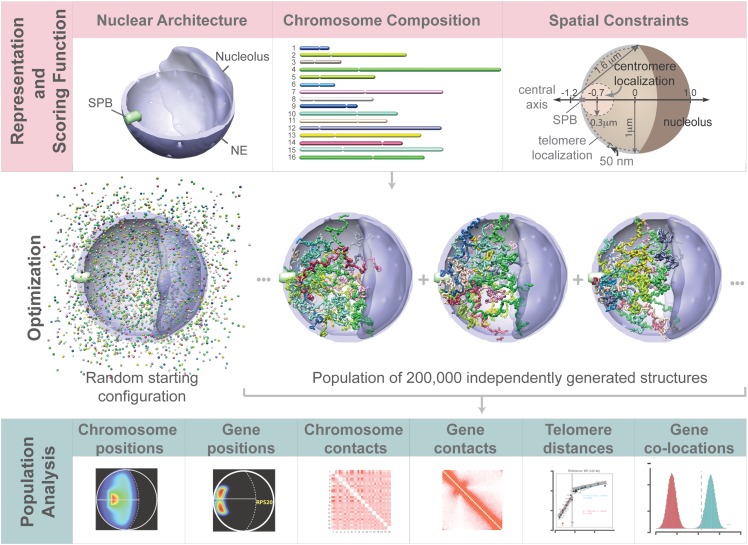
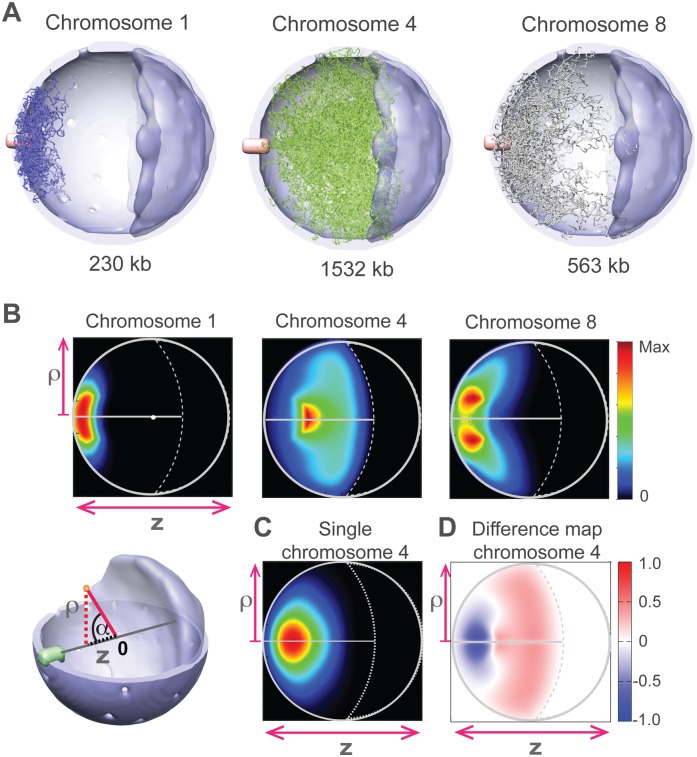
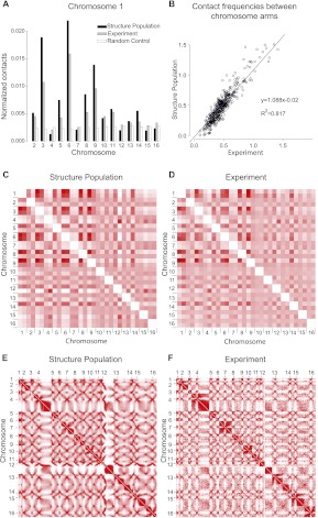
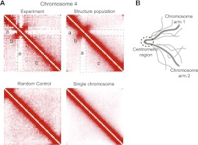
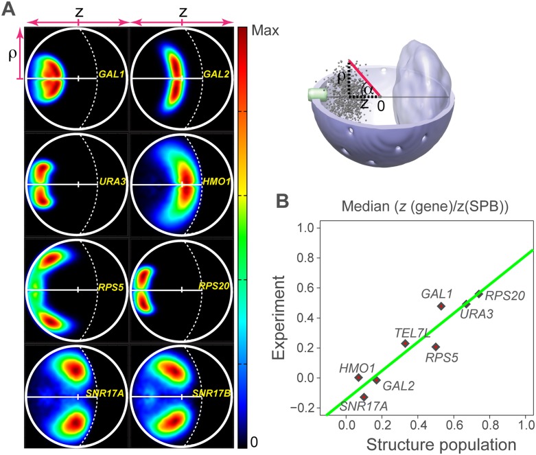
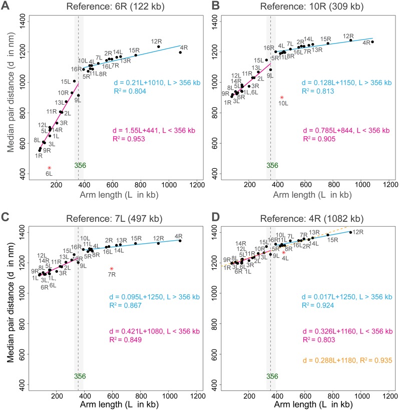
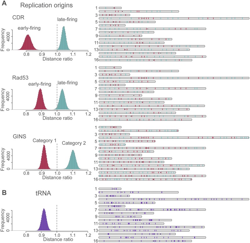
In this paper we show that tethering of heterochromatic regions to nuclear landmarks and random encounters of chromosomes in the confined nuclear volume are sufficient to explain the higher-order organization of the budding yeast genome. We have quantitatively characterized the contact patterns and nuclear territories that emerge when chromosomes are allowed to behave as constrained but otherwise randomly configured flexible polymer chains in the nucleus. Remarkably, this constrained random encounter model explains in a statistical manner the experimental hallmarks of the S. cerevisiae genome organization, including (1) the folding patterns of individual chromosomes; (2) the highly enriched interactions between specific chromatin regions and chromosomes; (3) the emergence, shape, and position of gene territories; (4) the mean distances between pairs of telomeres; and (5) even the co-location of functionally related gene loci, including early replication start sites and tRNA genes. Therefore, most aspects of the yeast genome organization can be explained without calling on biochemically mediated chromatin interactions. Such interactions may modulate the pre-existing propensity for co-localization but seem not to be the cause for the observed higher-order organization. The fact that geometrical constraints alone yield a highly organized genome structure, on which different functional elements are specifically distributed, has strong implications for the folding principles of the genome and the evolution of its function.


Figures

Figure 1.
Figure 1.
Population-based analysis of the S. cerevisiae genome organization. To analyze structural features of the genome, we defined an optimization problem with three main components. (Top panels) A structural representation of chromosomes as flexible chromatin fibers (center), a structural representation of the nuclear architecture (left), and the scoring function quantifying the genome structure's accordance with nuclear landmark constraints (right). (Middle panels) An optimization and sampling method, which minimizes the scoring function to generate a population of genome structures that entirely satisfies all landmark constraints. (Bottom panels) The statistical analysis and comparison of structural features from the population of 3D genome structures with all the experimental data.
Figure 2.
Figure 2.
Chromosome locations. (A) A sample of 40 chromosome configurations randomly selected from the structure population for the small chromosome 1 (left panel, blue chains), the large chromosome 4 (middle panel, green chains), and the medium-sized chromosome 8 (right panel, gray chains). The chain thickness is reduced to enhance visibility. The chromosomes are depicted in the nucleus with the SPB in pink, the nucleolus in dark blue, and the NE in light blue. (B, top) Chromosome localization probability densities (LPDs) of chromosomes 1 (left), 4 (middle), and 8 (right panel) plotted along the two principal axes ρ and z (Supplemental Material). (Lower left) Reference frame for projecting the positions of chromosome points onto the two principal axes, namely, the projection along the central axis z (connecting SPB, nuclear center, and nucleolus), and the radial distance ρ-axis indicating the absolute distance of a point from the central axis. (C) The LPD of chromosome 4 resulting from the “single chromosome population.” The chromosome is subject to all landmark constraints, but structures are generated without the presence of other chromosomes in the nucleus. The density distribution is significantly different from the situation when all chromosomes are present (see B). (D) Excluded volume effect. The difference map between the LPDs of chromosome 4 from the structure population when all chromosomes are present (B, middle) and the single chromosome population as defined in C.
Figure 3.
Figure 3.
Chromosome and gene loci interactions. (A) Histogram of the normalized contact frequencies of chromosome 1 with other chromosomes in the structure population (black bars), chromatin conformation capture experiments (gray bars) (Duan et al. 2010), and the random control population (white bars). Contact frequencies of other chromosomes are shown in Supplemental Fig. 2. (B) Comparison of chromosome-arm–chromosome-arm contact frequencies from the structure population and experiments (Duan et al. 2010). (C,D) Contact frequency heat maps for chromosome arm contacts in the structure population (C) and experiments (D) (Duan et al. 2010). Heat maps of the genome-wide contact frequencies between loci at 32-kb resolution determined from the structure population (E) and in a chromosome conformation capture experiment (F) (Duan et al. 2010). (Color code ranges from white for low to red for high values.) Centromere positions are marked by the ticks. The row-based average Pearson's correlation between the two heat maps is 0.94 (all P-values <10−6). The largest differences between both heat maps involve interactions to the small arm of chromosome 12, which is not surprising because it contains all of the rDNA genes located in the nucleolus, which are not explicitly treated in our simulation. To further improve these interactions it is necessary to include these regions in future simulations (see Supplemental Material).
Figure 4.
Figure 4.
Chromosome folding. (A) Heat maps showing intrachromosomal contact frequencies for chromosome 4 obtained from conformation capture experiments (top left) (Duan et al. 2010), structure population (top right), random control (bottom left), and single chromosome population (bottom right). The latter is derived from a structure population for a nucleus containing only chromosome 4, constrained in a manner identical to the full simulation. Heat maps of the experiment and the structure population show characteristic folding patterns reminiscent of the back-folding of subcentromeric regions onto themselves. The heat maps of the random control and the single chromosome population lack the characteristic pattern. (B) Scheme showing the particular back-folding of the regions adjacent to both sides of the centromere for several chromosome configurations.
Figure 5.
Figure 5.
Gene territories. (A) Projected localization probability densities for the positions of eight gene loci in the structure population. The probability densities are determined with respect to two principal axes of the nuclear architecture (top right panel). The z-axis connects the SPB with the origin at the nuclear center and the nucleolus. The radial axis ρ defines the distance of a point from the central axis (top right panel). The lower half of the projected localization density plot is mirrored from the top half for visual convenience. (B) Median gene loci position along the z-axis calculated from the projected probability localization densities in A and from the experiment (Berger et al. 2008). The two are highly correlated with R2 = 0.9. To allow for comparison with the experiment, the z-axis distance of a gene locus is normalized relative to the SPB–gene distance.
Figure 6.
Figure 6.
Median telomere–telomere distances in the structure population. The median distances between a telomere of a reference chromosome arm and all other telomeres are plotted for reference chromosome arms (A) 6R, (B) 10R, (C) 7R, and (D) 4R. (Vertical dashed line) Change point with 95% confidence interval shown by the shaded area.
Figure 7.
Figure 7.
Spatial clustering of replication origins and tRNA gene loci. (Left) The histograms show the distribution of the mean pair distance ratio between a set of specific sites (e.g., early replication sites) and all sites in the structures of the population. The histograms are generated as follows: For a given structure in the population, the mean pair distance between a set of specific loci (e.g., all early replication origins) is calculated. This distance is divided by the mean pair distance of all sites in the same structure. The distribution of the distance ratio is then obtained from all structures in the population. If the distribution is centered on 1 (vertical dashed line), the selected sites behave similarly to a random sample of all sites. If the distribution is shifted toward smaller values, their pair distances are smaller than would be expected from the background control. If the distribution is shifted to larger values, the selected sites are more distant from each other than would be expected from the random control background. (A) Distribution of distance ratios of early (red) and late (green) replication start sites as determined by three independent experiments using the CDR (Clb5 Dependent Region), Rad53 checkpoint-mediated regulation, and GINS complex as identifiers. For the latter case, category 1 sites start replication earlier than category 2 sites. (Right panel) The positions of each site in the chromosome sequence. The number of early- and late-firing sites labeled with CDR, Rad3, and GINS are 77 and 123, 101 and 99, and 169 and 135, respectively. (B) Distribution of distance ratios for all 275 tRNAs (loci extracted from SGD, http://www.yeastgenome.org). For all sets of sites in A and B, the shift of the mean pair distances is highly statistical significant (for details, see Supplemental Material and main text).

Similar articles

Cited by

References

    1. Alber F, Dokudovskaya S, Veenhoff LM, Zhang W, Kipper J, Devos D, Suprapto A, Karni-Schmidt O, Williams R, Chait BT, et al. 2007a. Determining the architectures of macromolecular assemblies. Nature 450: 683–694 - PubMed
    1. Alber F, Dokudovskaya S, Veenhoff LM, Zhang W, Kipper J, Devos D, Suprapto A, Karni-Schmidt O, Williams R, Chait BT, et al. 2007b. The molecular architecture of the nuclear pore complex. Nature 450: 695–701 - PubMed
    1. Alber F, Forster F, Korkin D, Topf M, Sali A 2008. Integrating diverse data for structure determination of macromolecular assemblies. Annu Rev Biochem 77: 443–477 - PubMed
    1. Berger AB, Cabal GG, Fabre E, Duong T, Buc H, Nehrbass U, Olivo-Marin JC, Gadal O, Zimmer C 2008. High-resolution statistical mapping reveals gene territories in live yeast. Nat Methods 5: 1031–1037 - PubMed
    1. Bohn M, Heermann DW 2010. Diffusion-driven looping provides a consistent framework for chromatin organization. PLoS ONE 5: e12218 doi: 10.1371/journal.pone.0012218 - PMC - PubMed

Publication types

MeSH terms

LinkOut - more resources