

Review
doi: 10.1021/cr100353t.
Epub 2011 Sep 16.
Structural analysis of macromolecular assemblies by electron microscopy
Affiliations
- PMID: 21919528
- PMCID: PMC3239172
- DOI: 10.1021/cr100353t
Item in Clipboard
Review
Structural analysis of macromolecular assemblies by electron microscopy
Chem Rev.
.
Free PMC article
No abstract available
Figures
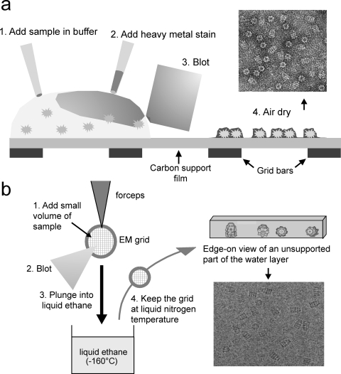
Negative stain and cryo EM sample preparation. (a) Schematic view of sample deposition, staining, and drying, with an example negative stain image. (b) Schematic of plunge freezing and of a vitrified layer, and an example cryo EM image. Panel (b) is adapted with permission from ref (24). Copyright 2000 International Union of Crystallography.
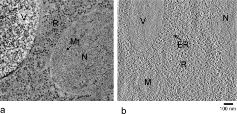
Slices of single axis tomograms of yeast cell sections prepared by freeze-substitution (a) and cryo-sectioning of vitrified samples (b). The black dots are mainly ribosomes. R, ribosomes; N, nucleus; V, vacuole; MT, microtubules (ring shaped cross sections); M, mitochondrion; ER, endoplasmic reticulum. Panel (b) was produced by Dan Clare.
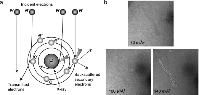
Interaction of the electron beam with the sample. (a) Schematic of elastic and inelastic electron scattering. Collision of beam electrons with atomic electrons or nuclei leads to energy loss (inelastic scattering), while deflection by the electron cloud does not change the energy of the electron (elastic scattering). (b) Effect of electron beam damage on a cryo image of a cell. The electron dose is shown on the images. Increasing dose causes damage to cellular structures, but different cell regions and materials show the effects of damage at different levels of radiation. In this case, damage first appears on the Weibel Palade bodies. Reproduced with permission from ref (54). Copyright 2009 National Academy of Sciences.
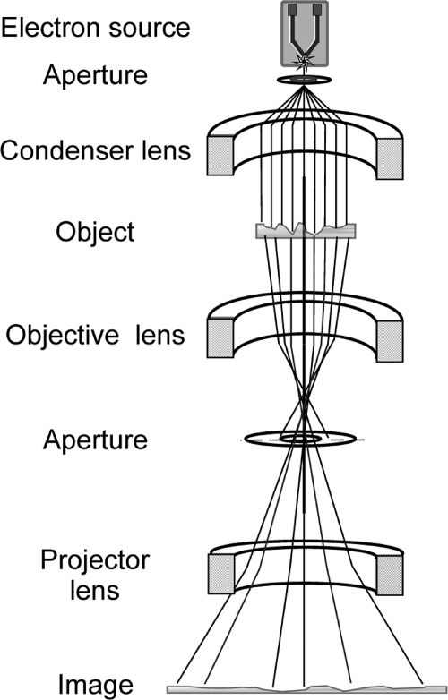
Simplified schematic representation of an electron microscope.
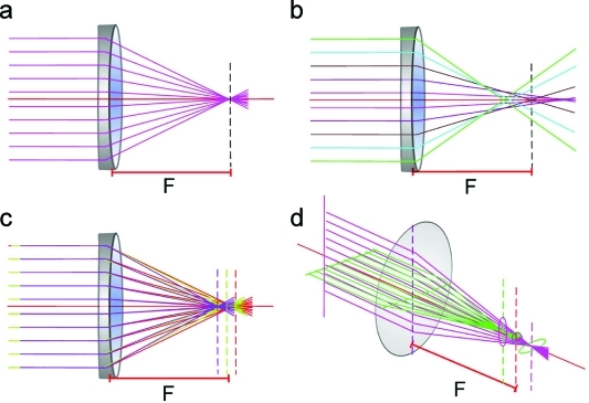
Ray diagrams of lens aberrations: (a) perfect lens, (b) spherical, (c) chromatic, and (d) astigmatic aberration. F is the focal length of the lens.
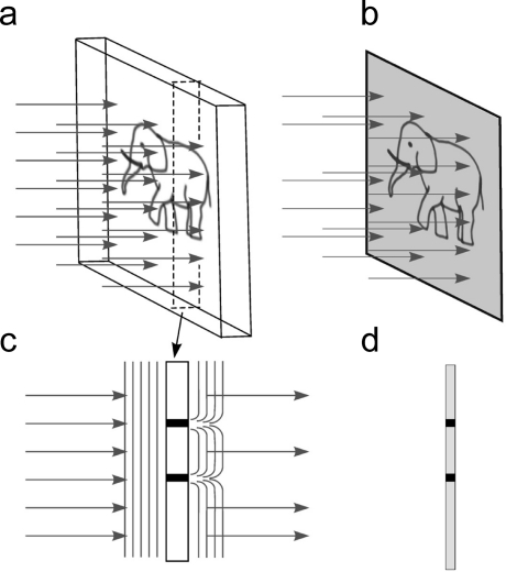
Amplitude contrast. (a) An amplitude object illuminated by a parallel beam. (b) The image resulting from interaction of the beam with the sample. (c) A cross section of the object outlined by the dashed lines in (a); some of the rays are absorbed in the sample. Arrows show the changes in the wavefront after interaction with the sample. (d) Intensity of the rays creating the image in the region of the cross section. Black dots in the image correspond to areas of beam absorption (c).
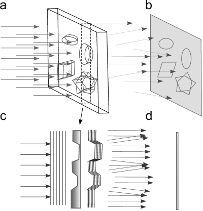
Phase contrast. (a) A phase object illuminated by a parallel beam. (b) The resulting image shows only weak features. (c) A cross section of the object outlined by dashed lines in (A). Arrows show the changes in the wavefront (parallel lines) after interaction with the sample. The intensity is not changed, but the wavefront becomes curved. (D) Intensity of the rays creating the image in the region of the cross section. Note that the intensity differences are small.
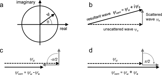
Graphical representation of phase contrast. (a) Complex plane representation of a wave vector ψ with phase θ. (b) Vector representation of the scattered wave ψs, unscattered wave ψu, and resultant wave ψsam = ψu + iψs. Amplitudes (vector lengths) of ψsam and ψu are very similar, resulting in low image contrast. (c) −π/2 phase shift of the scattered wave leads to a noticeable decrease in the resultant wave amplitude relative to the unscattered wave (negative phase contrast). (d) π/2 phase shift of the scattered wave increases the amplitude of the resultant wave relative to the unscattered wave (positive phase contrast).
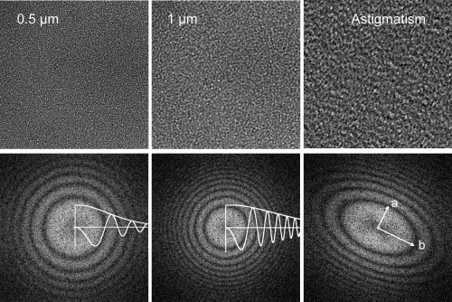
Images of carbon film and their diffraction patterns, showing Thon rings and corresponding CTF curves. The left image was obtained at 0.5 μm defocus, and the middle image was at 1 μm defocus. The Thon rings of the second image are located closer to the origin and oscillate more rapidly. The rings alternate between positive and negative contrast, as seen in the plotted curves. An example of an astigmatic image and its diffraction pattern is shown in the right panel. The largest defocus is along axis a, and the smallest is along axis b.
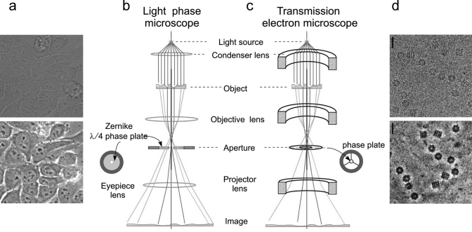
Phase contrast in optical and electron microscopy. (a) Bright field (upper panel) and phase contrast (lower panel) images of a field of cells. The cells are approximately 50 μm in length. Panel (a) was provided by Maud Dumoux and Richard Hayward. (b) Schematic representation of the light microscope. (c) Schematic representation of the electron microscope for comparison, showing the major lenses. The positions of phase plates are indicated. (d) Images of GroEL taken without (upper panel) and with the phase plate (lower panel). Scale bars, 20 nm. Image (d) is reproduced with permission from ref (67). Copyright 2008 Royal Society Publishing.
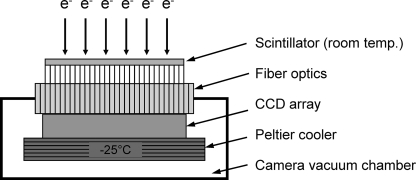
Diagram of a CCD detector for EM. The incident electrons are converted to photons by the scintillator. Fiber optics transmit the image to the CCD (charge coupled device) sensor where the photons generate electrical charge (CCD electrons). The charge is accumulated in parallel registers. During readout, this charge is shifted line by line to the serial register from where it is transferred pixel by pixel to the output analog-to-digital converter. Image reproduced with permission from H. Tietz.
Distortions caused by the missing wedge. (a) A model object. (b) Set of image planes at different angles from a tilt series. The limitation on maximum tilt angle results in a missing wedge of data. (c) Reconstruction of the object showing elongated features due to the missing wedge. Reproduced with permission from ref (99). Copyright 1998 Elsevier Inc.
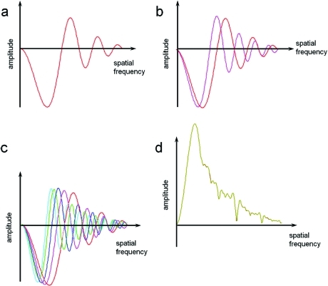
CTF curves, for a single defocus (a), overlaid for two different defocus values (b). The red curve corresponds to a closer to focus image, and oscillates more slowly. Image (c) shows multiple defocus values. The cyan/green curves correspond to the images with the highest defocus, and the red curve is closest to focus. (d) The sum of amplitude absolute values of all curves in (c), showing the overall transfer of spatial frequency components in a data set with the defocus distribution shown. Images courtesy of Neil Ranson.
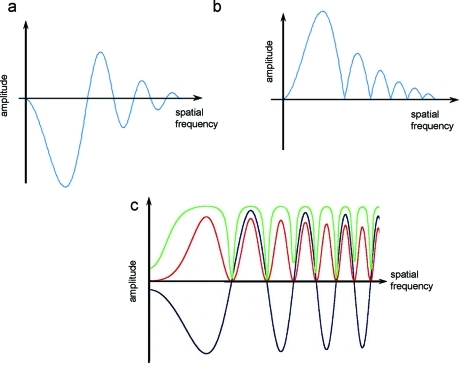
(a) CTF curve from uncorrected data, (b) after phase correction, and (c) overlay of original (black), the square of the curve after rescaling (red), and amplitude correction (green). Panel (c) courtesy of Stephen Fuller.
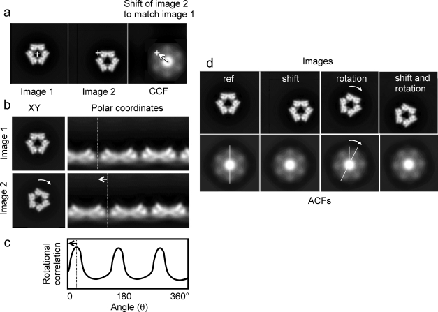
Alignment using translational and rotational cross correlations and autocorrelation. (a) Two images to be aligned, with the second shifted off center. The right panel shows the cross-correlation function (CCF) of the second image with the first. The crosses indicate the image centers. The arrow indicates the shift that must be applied to image 2 to bring it into alignment with image 1, according to the CCF maximum. (b) Two images, related by a 25° rotation, shown in Cartesian (left) and polar coordinates (right). The curved arrow shows the rotation in the Cartesian coordinate view, and the dashed line shows the corresponding shift of a feature in the polar coordinate representation. (c) Plot of the rotational correlation between the two images in (b). The arrow shows the angular shift required to align image 2 to image 1. (d) Images and their corresponding autocorrelation functions (ACF). When the image is shifted (second panel), the ACF is unchanged (translationally invariant). The reference image (ref) has 3-fold symmetry, but its ACF is 6-fold because of the centrosymmetric property of ACFs. Rotation of the image causes the same rotation of the ACF, but has an ambiguity of 180°. A possible alignment strategy is to use the ACF first for rotational alignment, using the property of translational invariance. The CCF then can be used for translational alignment, checking both 0° and 180° rotational positions.
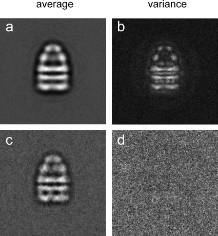
Average and variance for an image set of particles whose orientations are distributed by rotation around the symmetry axis (a,b) and for an image set of particles in a single orientation (c,d). The average in (a) contains images of particles in different orientations, resulting in significant variation of image features (b). Panel (d) is featureless, because all of the particles in the average (c) have the same orientation, so that the projections only differ in the noise background. Figure courtesy of Neil Ranson.
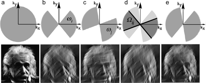
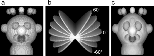
Diagrams of angular coverage and the corresponding images, to illustrate alignment of subtomograms taking account of the missing wedge. (a) The original image with no missing data. (b) The effect of a missing wedge along the y axis on the image. Only projections within the gray sector ωi are used to produce the image. Some features of the face (wrinkles and eyes) are not resolved. (c) Another set of projections ωj with the missing wedge in a different orientation causes different features to be lost. (d) If only the data common to the two images (b) and (c) are present (Ωij), the image is more distorted. Nevertheless, alignment of the two images (b and c) can be based on this overlapping information. Otherwise, the alignment would be biased by the missing wedge. (e) After alignment, the two data sets (b) and (c) can be combined to give a better angular coverage, so that the reconstruction more closely resembles the original object. Modified with permission from ref (134). Copyright 2008 Elsevier Inc.
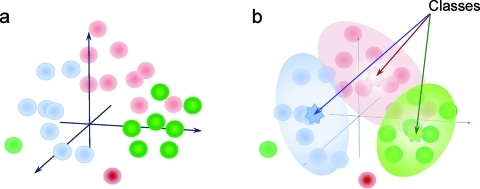
Schematic of a data cloud illustrating the principles of multivariate statistical analysis and classification. (a) Each image is represented by a color-coded dot in a multidimensional data cloud, which has been subjected to MSA. (b) The dots are sorted into three classes according to color and position. Several outlying dots (represented by inconsistency between color and position) are not assigned to major classes and represent classes composed only by one dot, and are not considered as representative classes.
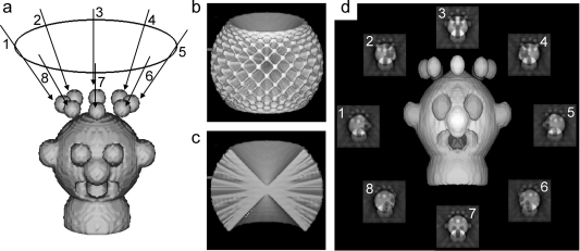
Conical tilt geometry. (a) The original object, with arrows indicating the angular directions of the data projections. (b) Representation of the sections in Fourier space corresponding to data projections collected within this cone of angles. A central cross section of the planes in Fourier space is shown in (c). (d) A surface view of the resulting conical tilt reconstruction, surrounded by the eight projections corresponding to the original view directions. Reproduced with permission from ref (99). Copyright 1998 Elsevier Inc.
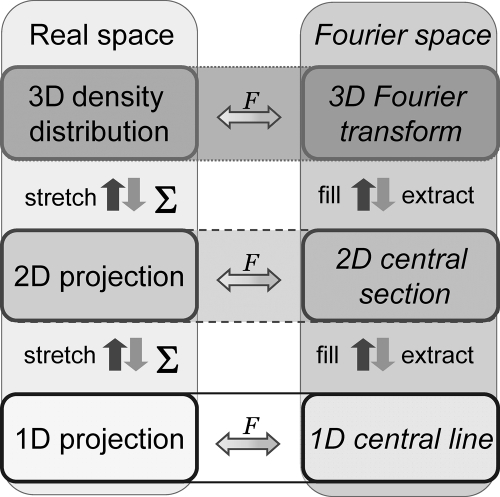
Relationships between images and projections in real and Fourier space. The 3D structure can be projected onto planes to give 2D projections, which can in turn be projected in different directions to yield 1D (line) projections, indicated by the operator of summation ∑. The complete set of line projections is known as the Radon transform. A sinogram is a set of line projections of the 2D projection or a section of the 3D Radon transform. In the reverse direction, the set of line projections can be combined to reconstruct the 2D image and the set of 2D projections combined to reconstruct the 3D object, indicated by the operator of stretching. The image information can be equivalently represented in reciprocal space, in the form of Fourier amplitudes and phases (right column). Fourier transforms (F) of the 2D projections correspond to central sections of the 3D transform (extraction), and the line projections correspond to lines passing through the origin of Fourier space (central lines). Therefore, the object can also be reconstructed by combining (filling) the set of central sections into the 3D transform followed by inverse 3D Fourier transformation. Adapted with permission from ref (12). Copyright 2000 Cambridge University Press.
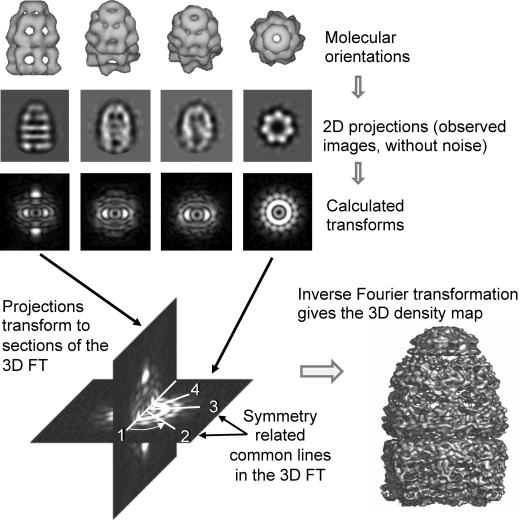
Surface rendered views, projections, and transform sections of a structure, with a common line intersection illustrated in reciprocal space. The structure has rotational symmetry, and there are several symmetry-related common lines. From the angles between common line projections of different views, the relative Euler-angle orientations of a set of projections can be determined. Adapted with permission from ref (24). Copyright 2000 International Union of Crystallography.
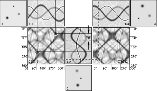
Sinograms and sinogram correlation functions for a model structure. Three projections (numbered 1–3) are shown of a model composed of three Gaussian dots with different densities. S1, S2, and S3 are sinograms or sets of 1D projections of the corresponding 2D projections. CSC12 and CSC32 represent cross-sinogram correlation functions between projections 1 and 2 and projections 3 and 2, respectively. Each point of the sinogram correlation function contains the correlation coefficient of a pair of lines from the two sinograms. Solid lines indicate the common lines between projections 2 and 1, while the dashed lines indicate the common lines between projections 2 and 3. Each CSC has two peaks because projections from 180° to 360° mirror those from 0° to 180°. The angular distance between the common lines (solid and dashed) gives the angle between projections 1 and 3.
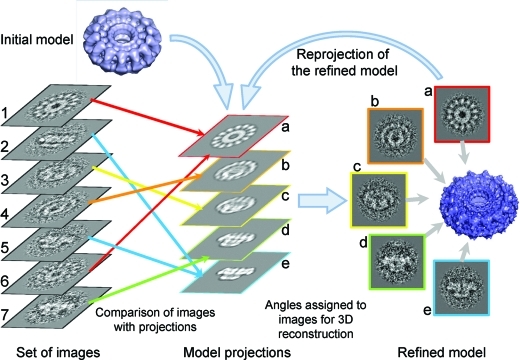
Projection matching procedure. A set of images is compared to a set of references from an initial model (low resolution). Once the best match is found between the image and one of the references (reprojections), based on the height of the correlation peak, the shift relative to the matching reference and angles of that reference are assigned to the image. Images 1 and 6 have the best correlation with model projection a (red arrows), while images 2 and 5 match image e (blue arrows). Image 3 corresponds to the tilted view c (yellow arrow). A new 3D map is calculated using images with the assigned angles. The refined 3D reconstruction is then reprojected with a smaller angular increment to generate new references for the next iteration of refinement.
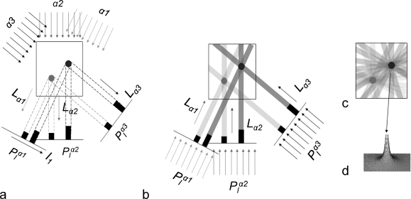
Back-projection algorithm. (a) Projections Plα1, Plα2, and Plα3 are obtained experimentally from an object containing two dots of different density. α1, α2, and α3 are the angles of the different projection directions, and Lα1, Lα2, and Lα3 are the unit vectors of the corresponding projection directions (eq 20). (b) Back projection is done by stretching projections back through the area to be reconstructed along the original projection directions, or in other words by creating rays of pixels with the density of the corresponding projection pixel. This is shown as light and dark gray lines from projections 1, 2, and 3. The rays are summed in the reconstructed area, providing information on the dot positions. (c) The more projections that are used, the better defined are the dots. (d) An artifact of the technique is that each point is surrounded by a background halo. The intensity of the halo is proportional to the density of the dot.

Filtered back projection. The original object contains two dots of different densities. The upper panel represents reconstructions by back projection of these dots using 7, 15, 45, and 180 projections, respectively. Although the radial streaks are eliminated by using more projections, this method leaves a halo around the reconstructed dots. The bottom panels show reconstructions from the same projections using filtering. Reduction of the halo is most pronounced on the reconstructions with more projections.
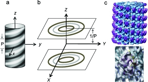
Fourier Bessel reconstruction. (a) A helical structure with a sinusoidal density profile of pitch P. (b) The Fourier transform of the helix (a) constitutes two planes on which the amplitudes are represented as concentric rings with phases alternating between 0° and 180°. The amplitudes of the rings are described by Bessel functions. (c) Reconstruction of a microtubule complexed with the kinesin-5 motor at a resolution 9 Å. Enlargement of the boxed area shows the fit of the X-ray structure into the EM map. Parts (a) and (b) are based on earlier figures by Moody.(19) Part (c) is reproduced with permission from ref (197). Copyright 2010 Elsevier Inc.
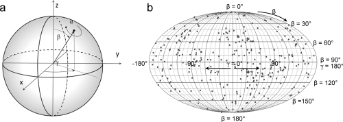
Euler sphere and distribution of projections. (a) The Euler sphere is an imaginary sphere of unit radius with the object located at its center. The points on its surface represent view directions of the object. A projection direction is shown by the vector from the center to the viewpoint on the sphere surface, so the angles of the projection are described by the vector direction. In this figure, the angle convention is as in IMAGIC α, β, and γ, corresponding to SPIDER angles ψ, θ, and φ, with ψ = 90° – α; θ = β; φ = γ – 90°. (b) An example of the angle distribution of a single-particle data set on the Euler sphere shown in elliptical (Mollweide) projection. This representation shows the angle of projection directions relative to the z axis (β angle) and around it (γ angle), but the rotation in the image plane is not shown. These figures are normally used to examine the angular distribution of images used for reconstruction, to assess the uniformity of spatial coverage in the data set.
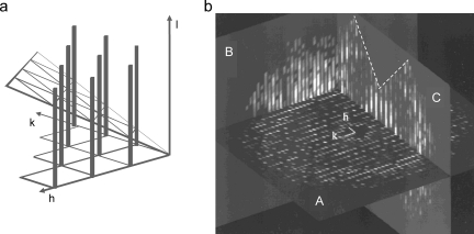
Electron crystallography. (a) Schematic diagram of lattice lines from a 2D crystal and their intersection with a tilted plane of data. Adapted from ref (198). Copyright 1982 Pergamon Press. (b) 3D electron diffraction pattern of a tubulin crystal. Plane A shows the untilted electron diffraction pattern, and planes B and C restore the lattice lines from the tilt series. The missing wedge can be seen on plane C (dashed lines). Unit vectors h and k indicate the position of the origin. Part (b) is reproduced with permission from ref (202). Copyright 2010 Elsevier Inc.
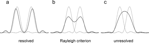
Resolution definition by separation of features. (a) When two points are far apart, there is a deep trough of density between them. (b) Two points are regarded as just resolved when the peak of one point spread function overlaps the first minimum of the other (Rayleigh criterion), see ref (60). (c) The point spread functions of two dots close together overlap to form one maximum, so that the points are not resolved.
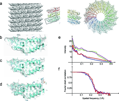
Effects of full CTF correction and amplitude scaling on the appearance and resolution of an EM map of TMV. (a) Surface view and two orthogonal central sections of an EM map of TMV, with the fitted atomic structure shown on the sections (ref (23)). (b) Enlargement of the boxed region in (a), of a map obtained only with phase correction but not amplitude correction or scaling. (c) The same map region after full amplitude correction. (d) The map region after full amplitude correction and B-factor scaling. (e) Rotationally averaged power spectra of the maps with phase correction (blue), amplitude and phase correction (red), of a map calculated from the atomic structure fit (green), and of the fully corrected and B-factor scaled map (purple). (f) FSC curves for the phase and amplitude corrected maps, colored as in (e). Reproduced with permission from ref (83). Copyright 2010 Elsevier Inc.
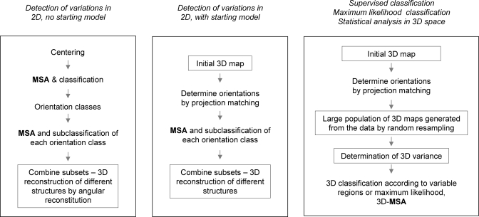
Three main approaches currently used to identify and sort molecular heterogeneity. The first approach (left panel) is based on statistical analysis of 2D images (a priori analysis) to detect the heterogeneity of the sample in its images. The initial sorting is done prior to any 3D reconstruction. The second approach (middle panel) requires an initial 3D map to separate the images into subsets according to their orientation. Analysis of structural heterogeneity is done in 2D for each orientation subset. The third method (a posteriori analysis) is based on examination of variations in multiple 3D maps (right panel). Reproduced with permission from ref (220). Copyright 2010 Elsevier Inc.
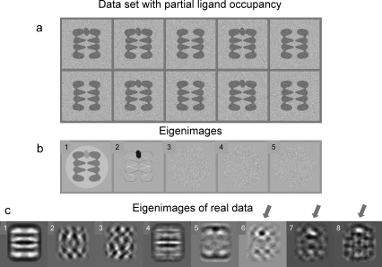
Statistical analysis to detect variable ligand occupancy. A model data set with variable ligand occupancy, simplified to show only one orientation (a), and the corresponding eigenimages (b). The first eigenimage is the sum of all images. The area corresponding to the ligand has density proportional to the occupancy (50%) of the ligand in the complex. The second eigenimage shows a very dark spot located in the area of the ligand. This feature reflects the major variation present in the data set. The remaining eigenimages reflect variations related to noise in the images. (c) Real eigenimages from a data set of GroEL with variable binding of non-native malate dehydrogenase. Eigenimages 2 and 3 show variations mainly related to different orientations around the rotation axis. Eigenimage 4 indicates small variations in tilt around a horizontal axis. Eigenimages 5–8 mainly reveal variations related to occupancy and location of the ligand in the complex (arrows). Reproduced with permission from ref (229). Copyright 2007 Elsevier Inc.
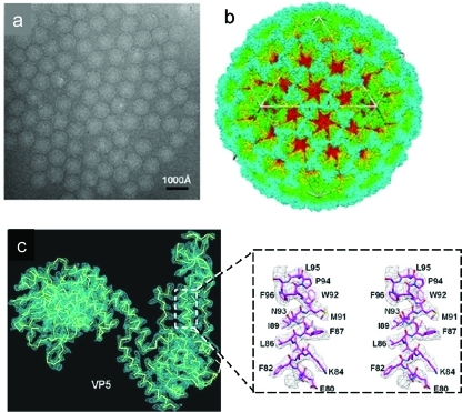
High-resolution single-particle EM of Aquarheovirus. (a) Raw images of viruses in vitreous ice. (b) 3D reconstruction colored according to radius. (c) Structure of subunit VP5 with the backbone model and enlargement to show side-chain detail. Reproduced with permission from ref (15). Copyright 2010 Elsevier Inc.
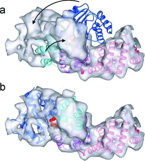
Flexible fitting of the crystal structure of the N-terminal part of the human apopotosome (domains NBD, HD1, WHD, and HD2) into the corresponding segmented cryoEM map at 9.5 Å resolution (ref (239)). (a) Initial fit before adjustment of the structure. (b) Result of flexible fitting. Figure courtesy of Shujun Yuan.
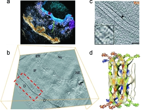
From a section of skin tissue to molecular shape of cadherin. (a) Segmented, rendered image showing the different cellular components in the reconstructed tissue section. (b) Tomogram slice. D, desmosome; IF, intermediate filaments; Nu, nucleus; ER, endoplasmic reticulum; NE, nuclear envelope; Mi, mitochondrion. (c) Desmosome extracted from the area in the red dashed box in (b), with an inset of the averaged image. (d) Sub tomogram average with fitted cadherins. Reproduced with permission from ref (242). Copyright 2007 Macmillan Press.
Similar articles
-
Metal shadowing and decoration in electron microscopy of biological macromolecules.Ann N Y Acad Sci. 1986;483:57-76. doi: 10.1111/j.1749-6632.1986.tb34497.x. Ann N Y Acad Sci. 1986. PMID: 2436521 No abstract available.
-
Determining the structure of biological macromolecules by transmission electron microscopy, single particle analysis and 3D reconstruction.Prog Biophys Mol Biol. 2001;75(3):121-64. doi: 10.1016/s0079-6107(01)00004-9. Prog Biophys Mol Biol. 2001. PMID: 11376797 Review.
-
Survey of the analysis of continuous conformational variability of biological macromolecules by electron microscopy.Acta Crystallogr F Struct Biol Commun. 2019 Jan 1;75(Pt 1):19-32. doi: 10.1107/S2053230X18015108. Epub 2019 Jan 1. Acta Crystallogr F Struct Biol Commun. 2019. PMID: 30605122 Free PMC article. Review.
-
Low temperature electron microscopy.Annu Rev Biophys Bioeng. 1981;10:133-49. doi: 10.1146/annurev.bb.10.060181.001025. Annu Rev Biophys Bioeng. 1981. PMID: 7020572 Review. No abstract available.
-
Structural studies by electron tomography: from cells to molecules.Annu Rev Biochem. 2005;74:833-65. doi: 10.1146/annurev.biochem.73.011303.074112. Annu Rev Biochem. 2005. PMID: 15952904 Review.
Cited by
-
(Cryo)Transmission Electron Microscopy of Phospholipid Model Membranes Interacting with Amphiphilic and Polyphilic Molecules.Polymers (Basel). 2017 Oct 19;9(10):521. doi: 10.3390/polym9100521. Polymers (Basel). 2017. PMID: 30965829 Free PMC article. Review.
-
Membranes under the Magnetic Lens: A Dive into the Diverse World of Membrane Protein Structures Using Cryo-EM.Chem Rev. 2022 Sep 14;122(17):13989-14017. doi: 10.1021/acs.chemrev.1c00837. Epub 2022 Jul 18. Chem Rev. 2022. PMID: 35849490 Free PMC article. Review.
-
Isotropic reconstruction for electron tomography with deep learning.Nat Commun. 2022 Oct 29;13(1):6482. doi: 10.1038/s41467-022-33957-8. Nat Commun. 2022. PMID: 36309499 Free PMC article.
-
Assembly of macromolecular complexes by satisfaction of spatial restraints from electron microscopy images.Proc Natl Acad Sci U S A. 2012 Nov 13;109(46):18821-6. doi: 10.1073/pnas.1216549109. Epub 2012 Oct 29. Proc Natl Acad Sci U S A. 2012. PMID: 23112201 Free PMC article.
-
Cryogenic superresolution correlative light and electron microscopy on the frontier of subcellular imaging.Biophys Rev. 2021 Nov 26;13(6):1163-1171. doi: 10.1007/s12551-021-00851-4. eCollection 2021 Dec. Biophys Rev. 2021. PMID: 35059034 Free PMC article. Review.
References
-
- Dubochet J.; Adrian M.; Chang J. J.; Homo J. C.; Lepault J.; McDowall A. W.; Schultz P. Q. Rev. Biophys. 1988, 21, 129. - PubMed
Publication types
MeSH terms
Substances
Grants and funding
LinkOut - more resources
Full Text Sources
