. 2009 Dec;168(3):378-87.
doi: 10.1016/j.jsb.2009.08.016. Epub 2009 Sep 2.

CTF determination and correction for low dose tomographic tilt series

Affiliations

CTF determination and correction for low dose tomographic tilt series

Quanren Xiong et al. J Struct Biol. 2009 Dec.

Abstract

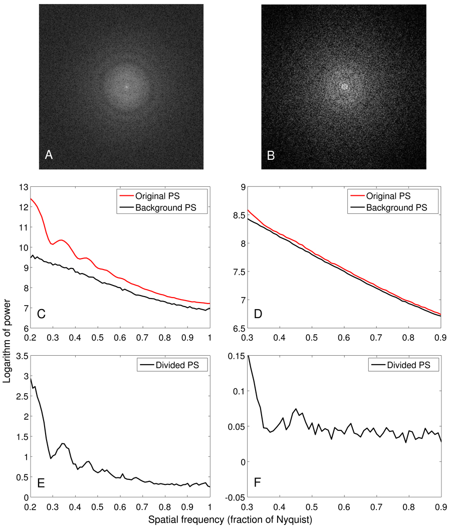
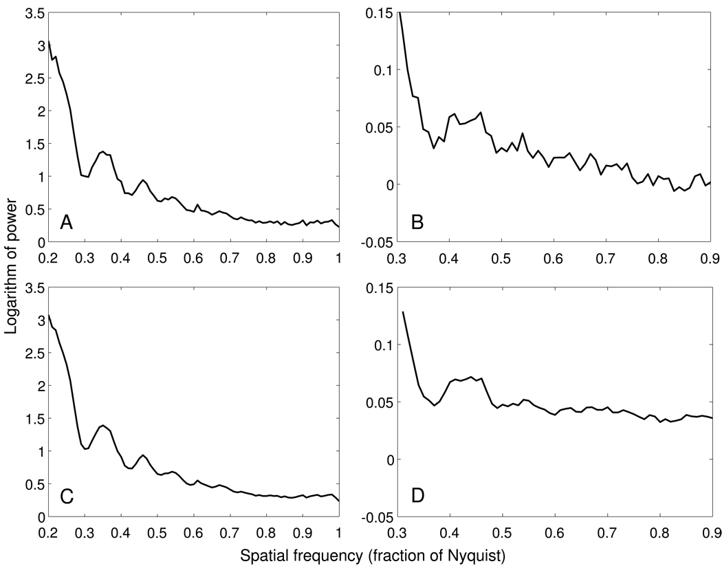
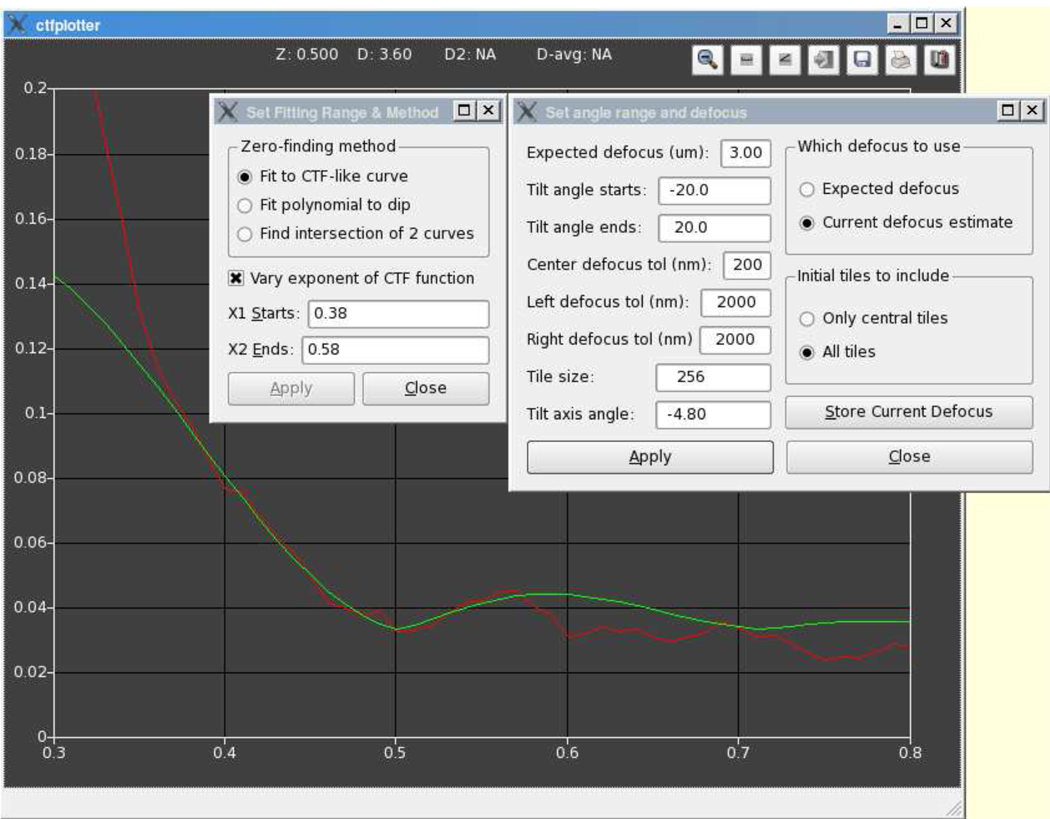
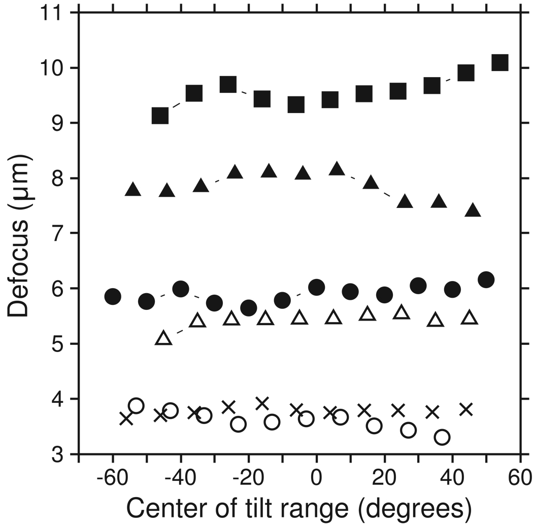
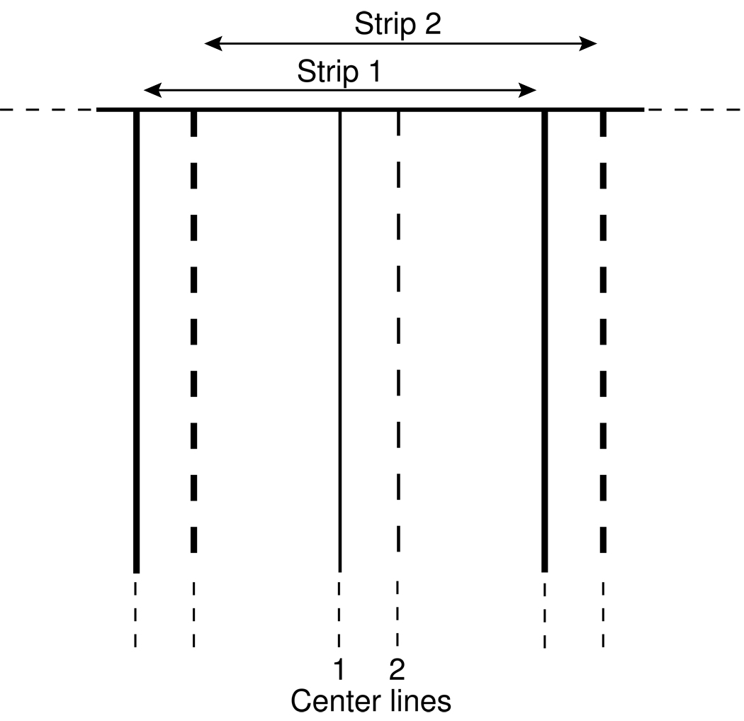
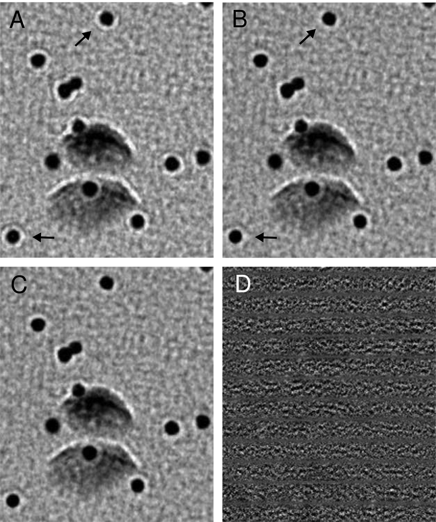
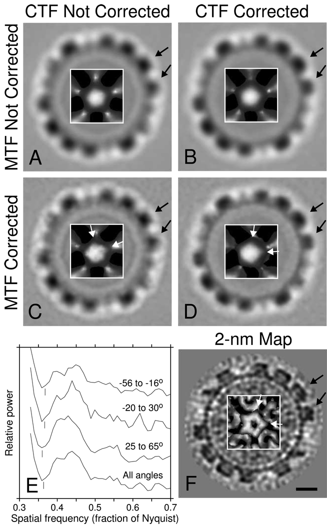
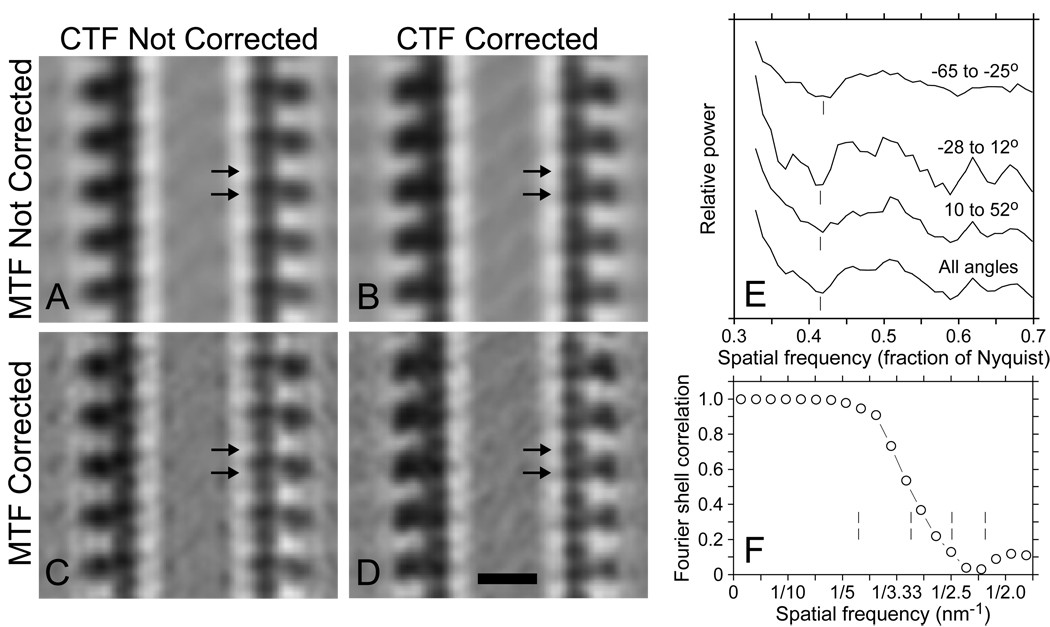
The resolution of cryo-electron tomography can be limited by the first zero of the microscope's contrast transfer function (CTF). To achieve higher resolution, it is critical to determine the CTF and correct its phase inversions. However, the extremely low signal-to-noise ratio (SNR) and the defocus gradient in the projections of tilted specimens make this process challenging. Two programs, CTFPLOTTER and CTFPHASEFLIP, have been developed to address these issues. CTFPLOTTER obtains a 1D power spectrum by periodogram averaging and rotational averaging and it estimates the noise background with a novel approach, which uses images taken with no specimen. The background-subtracted 1D power spectra from image regions at different defocus values are then shifted to align their first zeros and averaged together. This averaging improves the SNR sufficiently that it becomes possible to determine the defocus for subsets of the tilt series rather than just the entire series. CTFPHASEFLIP corrects images line-by-line by inverting phases appropriately in thin strips of the image at nearly constant defocus. CTF correction by these methods is shown to improve the resolution of aligned, averaged particles extracted from tomograms. However, some restoration of Fourier amplitudes at high frequencies is important for seeing the benefits from CTF correction.


Figures

Figure 1
Figure 1
Power spectra for images from tilt series taken at a high dose over a carbon support film (left column: dose 10 e2, 10 µm underfocus, ice-embedded specimen) and a low dose over a hole in the film (right column: dose 1 e2, 9 µm underfocus). A, B: FFTs of 0° tilt images. C, D: Logarithms of the original and background power spectra for tiles from these images. E, F: Logarithms of the original power spectrum divided by the background power spectrum.
Figure 2
Figure 2
Rotationally averaged power spectra obtained using tiles from images at tilt angles from 30° to 45° in the high and low dose tilt series used for Figure 1. A, B. Power spectra based on tiles whose defocus is within 200 nm of the defocus at the center of the image. C, D. Power spectra resulting from adding in tiles at higher defocus difference, after shifting their power spectra as described in the text.
Figure 3
Figure 3
User interface of the CTFPLOTTER program. The red curve is the averaged power spectrum, whose computation is controlled by the parameters in the right dialog box. The only text fields that the general user needs to modify are the expected defocus and the limiting tilt angles; the rest are available for experimentation. The radio buttons control whether to compute the power spectrum from just central tiles or from all tiles, and which defocus to assume when shifting off-center power spectra into register with central ones. Using the current defocus estimate allows one to iterate rapidly until the estimate converges. The green curve is fit to the power spectrum, based on the parameters in the left dialog box, which allows one to select the kind of curve(s) to fit and the range of frequencies over which to fit (see text for details). The “Z” and “D” outputs at the top of the window show the relative frequency and defocus of the first zero. These values are set each time that curve-fitting is done, but can be changed by clicking at a desired x coordinate. If the position of the second zero is clear, the user can click on it with a different mouse button and the “D2” and “D-avg” outputs will show the defocus based on that zero and the average of that with the defocus based on the first zero.
Figure 4
Figure 4
Plots of defocus versus tilt angle for 6 tilt series, showing that systematic changes in defocus do occur and can be detected with our approach. Values were obtained by fitting a CTF-like curve to power spectra from a 20° or 10° angular range at 10° intervals. The frequency fitting range was set from an initial power spectrum over a 40° range around zero tilt and then applied to all other angular ranges, requiring modification in only one case. The tilt series were of BPV and taken on the F20 (filled squares, open circles); of Eg5-decorated microtubules taken on the F20 (filled triangles); and of the ventral disk of Giardia taken on the F30 with energy filtering (filled circles, open triangles, crosses). One of the latter had such a good CTF signal that it was analyzed successfully with 10° ranges (filled circles). The entire angular range was analyzed for all sets except the low-defocus BPV set (open circles), where the power spectrum was too slanted in the last subrange.
Figure 5
Figure 5
Representation of adjacent strips used to speed up the line-by-line approach for correcting CTF. Strips 1 and 2 are transformed, corrected, and inverse transformed; these data are used to correct all lines between the center lines of the two strips. The lines are parallel to the tilt axis, which is vertical in the aligned images that are corrected.
Figure 6
Figure 6
Difference between correcting using a line-by-line method and using strip-based correction with interpolation between strips. A) Original projection image of 10-nm colloidal gold particles on a carbon film tilted to 65°. The image was taken on an F30 at 5.7 µm underfocus and the region shown is at 6.5 µm defocus. The tilt axis is horizontal in these images. B) Image corrected one line at a time. The effect of the correction is difficult to see when comparing images side-by-side, but the underfocus fringes around the gold particles are noticeably reduced (arrows). (The fringes remaining after correction reflect the dominance of frequencies below the first zero of the CTF.) C) Image corrected by interpolating between corrected strips 20 pixels apart. D) Difference between the images in B and C, showing no organized features related to the structure. The difference is less than 0.5% of the original intensity range, and it would appear uniformly gray if shown at the same intensity scaling as the images.
Figure 7
Figure 7
Averages of bovine papilloma virus (BPV) from a tilt series taken at 9.6 µm underfocus, based on 4000 aligned orientations of a subset of 519 virus particles. Each panel shows an image slice near the equator of the virus and an inset with a surface rendering of a capsomere at a 5-fold vertex. A. Average from tomogram without CTF correction. B. Average from tomogram after CTF correction of the tilt series. C. Average without CTF correction, filtered by the inverse of the camera MTF to restore high frequency information. D. Average with CTF correction and inverse filtering by the MTF. F. Map at 2-nm resolution [12] used for Fourier shell correlation with the averages. Black arrows mark capsomeres that are more appropriately shaped after CTF correction; the difference is slight between A and B but more noticeable between C and D. White arrows point to the vertices of the pentamer at the 5-fold vertex; the orientation of the pentamer is clearly incorrect in C. E. Power spectra used to determine the defocus for CTF correction for three angular subranges of the tilt series, and the power spectrum based on the whole tilt series. The curves are displaced vertically by arbitrary amounts. Vertical lines mark the frequencies manually chosen for the zeros, corresponding to 9.55, 9.6, and 9.85 µm underfocus for −56° to −16°, −20° to 30°, and 25° to 65°, respectively. The scale bar in F corresponds to 10 nm in the main images and 6 nm in the insets.
Figure 8
Figure 8
A. Fourier shell correlation between averages of BPV from tomograms and the 2-nm map, showing the phase inversion before CTF correction. The FSC is computed using the real component of the conjugate product of corresponding Fourier components. Vertical dashed lines show the locations of the first four zeros of the CTF. B, C. FSC values at 4 spatial frequencies near CTF zeroes, as a function of the defocus assumed when computing the CTF correction. The curves indicate that the best correction overall was obtained with the measured defocus, and that an error of 0.25 µm has relatively little impact on the value of the correction.
Figure 9
Figure 9
Averages from a microtubule decorated with Eg5, obtained by aligning and averaging subunits from a microtubule in a tomogram generated from a tilt series taken at 7.4 µm underfocus. A. Average without CTF correction. B. Average with CTF correction of tilt series. C. Uncorrected average filtered by the inverse of the CCD camera MTF. D. Inverse-filtered, corrected average. In addition to the obvious differences in the appearance of the Eg5 heads, note that both tubulin subunits show up clearly after both corrections in D (arrows) but are less distinct before CTF correction and appear displaced in A and C because of the phase inversion of 4-nm information. E. Power spectra used to determine the defocus for CTF correction, as in Fig 7. Vertical lines mark the frequencies manually chosen for the zeros, corresponding to 7.15, 7.4, and 7.5 µm underfocus for −65° to −25°, −28° to 12°, and 10° to 52°, respectively. F. Fourier shell correlation between averages based on two halves of the data; vertical lines show the location of CTF zeros. Bar = 10 nm.

Similar articles

Cited by

References

    1. Zhu J, Penczek PA, Schroder R, Frank J. Three-dimensional reconstruction with contrast transfer function correction from energy-filtered cryoelectron micrographs: procedure and application to the 70S Escherichia coli ribosome. J. Struct. Biol. 1997;118:197–219. - PubMed
    1. Toyoshima C, Unwin N. Contrast transfer for frozen-hydrated specimens: determination from pairs of defocused images. Ultramicroscopy. 1988;25:279–291. - PubMed
    1. Thon F. Zur Defokussierungsabhangigkeit des Phasenkontrastes bei der elektronenmikroskopischen Abbildung. Z. Naturforshung. 1966:476–478.
    1. Henderson R, Baldwin JM, Downing KH, Lepault J, Zemlin F. Structure of purple membrane from halobacterium-halobium, recording, measurement and evaluation of electron-micrographs at 3.5 Å resolution. Ultramicroscopy. 1986;19:147–178.
    1. Fernandez J-J, Sanjurjo JR, Carazo J-M. A spectral estimation approach to contrast transfer function detection in electron microscopy. Ultramicroscopy. 1997;68:267–295.

Publication types

LinkOut - more resources