On the analysis of sedimentation velocity in the study of protein complexes
- PMID: 19644686
- PMCID: PMC2755746
- DOI: 10.1007/s00249-009-0514-1
On the analysis of sedimentation velocity in the study of protein complexes
Abstract
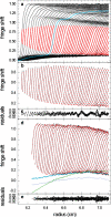
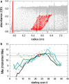
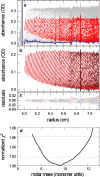
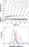
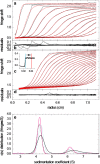
Sedimentation velocity analytical ultracentrifugation has experienced a significant transformation, precipitated by the possibility of efficiently fitting Lamm equation solutions to the experimental data. The precision of this approach depends on the ability to account for the imperfections of the experiment, both regarding the sample and the instrument. In the present work, we explore in more detail the relationship between the sedimentation process, its detection, and the model used in the mathematical data analysis. We focus on configurations that produce steep and fast-moving sedimentation boundaries, such as frequently encountered when studying large multi-protein complexes. First, as a computational tool facilitating the analysis of heterogeneous samples, we introduce the strategy of partial boundary modeling. It can simplify the modeling by restricting the direct boundary analysis to species with sedimentation coefficients in a predefined range. Next, we examine factors related to the experimental detection, including the magnitude of optical aberrations generated by out-of-focus solution columns at high protein concentrations, the relationship between the experimentally recorded signature of the meniscus and the meniscus parameter in the data analysis, and the consequences of the limited radial and temporal resolution of the absorbance optical scanning system. Surprisingly, we find that large errors can be caused by the finite scanning speed of the commercial absorbance optics, exceeding the statistical errors in the measured sedimentation coefficients by more than an order of magnitude. We describe how these effects can be computationally accounted for in SEDFIT and SEDPHAT.
Figures



Similar articles
-
Diffusion of the reaction boundary of rapidly interacting macromolecules in sedimentation velocity.Biophys J. 2010 Jun 2;98(11):2741-51. doi: 10.1016/j.bpj.2010.03.004. Biophys J. 2010. PMID: 20513419 Free PMC article.
-
Tools for the quantitative analysis of sedimentation boundaries detected by fluorescence optical analytical ultracentrifugation.PLoS One. 2013 Oct 18;8(10):e77245. doi: 10.1371/journal.pone.0077245. eCollection 2013. PLoS One. 2013. PMID: 24204779 Free PMC article.
-
Characterizing protein-protein interactions by sedimentation velocity analytical ultracentrifugation.Curr Protoc Immunol. 2008 May;Chapter 18:18.15.1-18.15.39. doi: 10.1002/0471142735.im1815s81. Curr Protoc Immunol. 2008. PMID: 18491296
-
Analytical ultracentrifugation for the study of protein association and assembly.Curr Opin Chem Biol. 2006 Oct;10(5):430-6. doi: 10.1016/j.cbpa.2006.08.017. Epub 2006 Aug 28. Curr Opin Chem Biol. 2006. PMID: 16935549 Review.
-
Evaluating the stoichiometry of macromolecular complexes using multisignal sedimentation velocity.Methods. 2011 May;54(1):39-55. doi: 10.1016/j.ymeth.2011.01.002. Epub 2011 Jan 20. Methods. 2011. PMID: 21256217 Free PMC article. Review.
Cited by
-
Recorded scan times can limit the accuracy of sedimentation coefficients in analytical ultracentrifugation.Anal Biochem. 2013 Jun 1;437(1):104-8. doi: 10.1016/j.ab.2013.02.011. Epub 2013 Feb 28. Anal Biochem. 2013. PMID: 23458356 Free PMC article.
-
Analytical Ultracentrifugation as a Tool for Studying Protein Interactions.Biophys Rev. 2013 Jun 1;5(2):159-171. doi: 10.1007/s12551-013-0106-2. Biophys Rev. 2013. PMID: 23682298 Free PMC article.
-
The association−dissociation behavior of the ApoE proteins: kinetic and equilibrium studies.Biochemistry. 2010 Nov 9;49(44):9533-41. doi: 10.1021/bi101407m. Biochemistry. 2010. PMID: 20923231 Free PMC article.
-
Sedimentation patterns of rapidly reversible protein interactions.Biophys J. 2010 May 19;98(9):2005-13. doi: 10.1016/j.bpj.2009.12.4336. Biophys J. 2010. PMID: 20441765 Free PMC article.
-
Accounting for solvent signal offsets in the analysis of interferometric sedimentation velocity data.Macromol Biosci. 2010 Jul 7;10(7):736-45. doi: 10.1002/mabi.200900456. Macromol Biosci. 2010. PMID: 20480511 Free PMC article.
References
-
- Balbo A, Brown P et al (2007) Step-by-step protocol for sedimentation velocity analytical ultracentrifugation. http://www.analyticalultracentrifugation.com/svprotocols.htm
-
- {'text': '', 'ref_index': 1, 'ids': [{'type': 'DOI', 'value': '10.1073/pnas.0408399102', 'is_inner': False, 'url': 'https://doi.org/10.1073/pnas.0408399102'}, {'type': 'PMC', 'value': 'PMC538923', 'is_inner': False, 'url': 'https://pmc.ncbi.nlm.nih.gov/articles/PMC538923/'}, {'type': 'PubMed', 'value': '15613487', 'is_inner': True, 'url': 'https://pubmed.ncbi.nlm.nih.gov/15613487/'}]}
- Balbo A, Minor KH et al (2005) Studying multi-protein complexes by multi-signal sedimentation velocity analytical ultracentrifugation. Proc Natl Acad Sci USA 102:81–86 - PMC - PubMed
-
- {'text': '', 'ref_index': 1, 'ids': [{'type': 'DOI', 'value': '10.1016/S0301-4622(01)00248-4', 'is_inner': False, 'url': 'https://doi.org/10.1016/s0301-4622(01)00248-4'}, {'type': 'PubMed', 'value': '11880173', 'is_inner': True, 'url': 'https://pubmed.ncbi.nlm.nih.gov/11880173/'}]}
- Behlke J, Ristau O (2002) A new approximate whole boundary solution of the Lamm differential equation for the analysis of sedimentation velocity experiments. Biophys Chem 95(1):59–68 - PubMed
-
- {'text': '', 'ref_index': 1, 'ids': [{'type': 'DOI', 'value': '10.1208/aapsj080368', 'is_inner': False, 'url': 'https://doi.org/10.1208/aapsj080368'}, {'type': 'PMC', 'value': 'PMC2761066', 'is_inner': False, 'url': 'https://pmc.ncbi.nlm.nih.gov/articles/PMC2761066/'}, {'type': 'PubMed', 'value': '17025277', 'is_inner': True, 'url': 'https://pubmed.ncbi.nlm.nih.gov/17025277/'}]}
- Berkowitz SA (2006) Role of analytical ultracentrifugation in assessing the aggregation of protein biopharmaceuticals. AAPS J 8(3):E590–E605 - PMC - PubMed
-
- {'text': '', 'ref_index': 1, 'ids': [{'type': 'DOI', 'value': '10.1529/biophysj.106.081372', 'is_inner': False, 'url': 'https://doi.org/10.1529/biophysj.106.081372'}, {'type': 'PMC', 'value': 'PMC1471869', 'is_inner': False, 'url': 'https://pmc.ncbi.nlm.nih.gov/articles/PMC1471869/'}, {'type': 'PubMed', 'value': '16565040', 'is_inner': True, 'url': 'https://pubmed.ncbi.nlm.nih.gov/16565040/'}]}
- Brown PH, Schuck P (2006) Macromolecular size-and-shape distributions by sedimentation velocity analytical ultracentrifugation. Biophys J 90:4651–4661 - PMC - PubMed
Publication types
MeSH terms
Substances
Grants and funding
LinkOut - more resources
Full Text Sources

