. 2009 Feb 26;61(4):635-48.
doi: 10.1016/j.neuron.2009.02.005.

Balanced amplification: a new mechanism of selective amplification of neural activity patterns

Affiliations

Balanced amplification: a new mechanism of selective amplification of neural activity patterns

Brendan K Murphy et al. Neuron. .

Erratum in

  • Neuron. 2016 Jan 6;89(1):235

Abstract

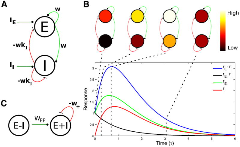
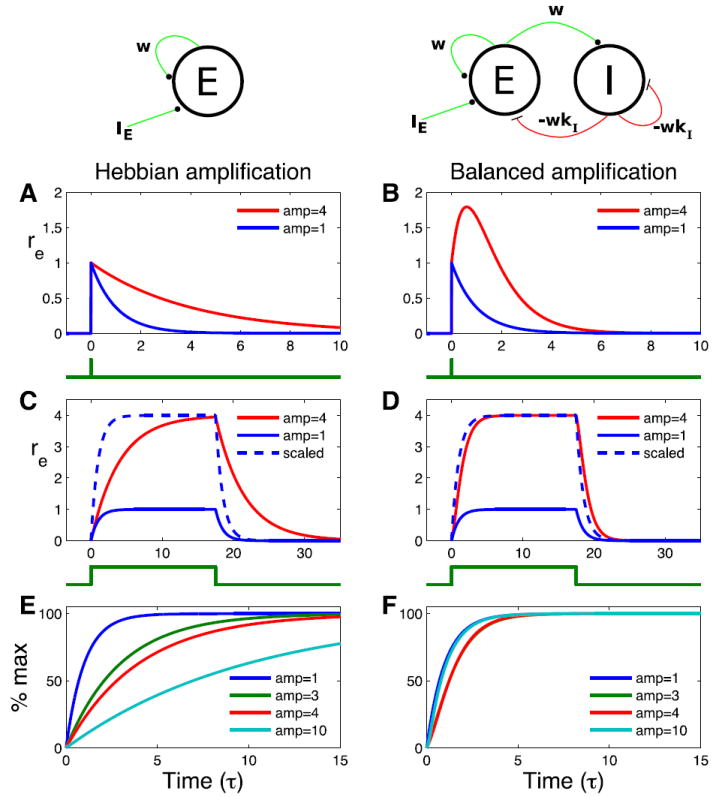
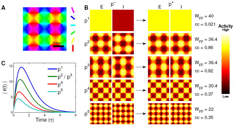
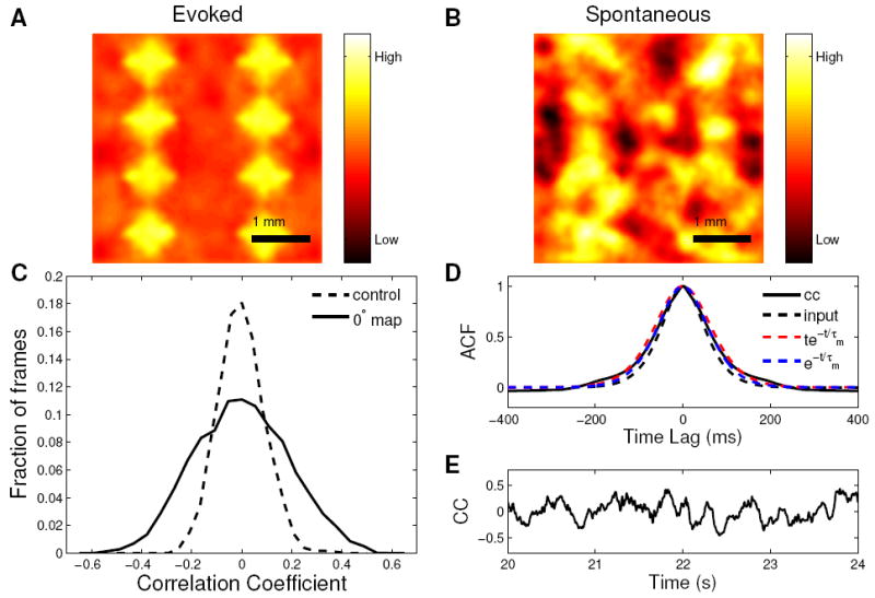
In cerebral cortex, ongoing activity absent a stimulus can resemble stimulus-driven activity in size and structure. In particular, spontaneous activity in cat primary visual cortex (V1) has structure significantly correlated with evoked responses to oriented stimuli. This suggests that, from unstructured input, cortical circuits selectively amplify specific activity patterns. Current understanding of selective amplification involves elongation of a neural assembly's lifetime by mutual excitation among its neurons. We introduce a new mechanism for selective amplification without elongation of lifetime: "balanced amplification." Strong balanced amplification arises when feedback inhibition stabilizes strong recurrent excitation, a pattern likely to be typical of cortex. Thus, balanced amplification should ubiquitously contribute to cortical activity. Balanced amplification depends on the fact that individual neurons project only excitatory or only inhibitory synapses. This leads to a hidden feedforward connectivity between activity patterns. We show in a detailed biophysical model that this can explain the cat V1 observations.


Figures

Figure 1
Figure 1. Balanced amplification in the two population case
A) Diagram of a balanced circuit with an excitatory and an inhibitory population. Excitatory connections are green and inhibitory connections are red. B) Plot of the sum (blue line) and difference (black line) between activity in the excitatory (rE, green line) and inhibitory (rI, red line) populations in response to a pulse of input to the excitatory population at time 0 that sets rE (0) = 1 (rI (0) = 0). Diagrams above the plot represent the color-coded levels of activity in the excitatory and inhibitory populations at the time points indicated by the dashed lines. C) The circuit depicted in A can be thought of as equivalent to a feedforward network, connecting difference activity pattern to sum activity pattern with strength wFF = w(1+kI). In addition, the sum pattern inhibits itself with strength w+ = w(kI − 1). Parameters: kI = 1.1; w=427 (for reasons explained in Fig. 2 legend).
Figure 2
Figure 2. Amplification of response to a pulse input and a sustained input
The firing rate response rE of the excitatory population to an external input IE to the excitatory population, in two models. Left column: The excitatory population makes a recurrent connection of strength w to itself, leading to Hebbian amplification. Right column: Balanced network as in Fig. 1, kI = 1.1. In all panels, blue lines show case without recurrent connections (w = 0). A, B) response to a pulse of input at time 0 that sets rE (0) = 1. Time course of input is shown below plots. Red curve shows response with weights set so that integral of response curve is 4 times greater than integral of blue curve (A, w = 0.75; B, w=427). C, D) Response to a sustained input IE = 1 (time course of input shown7). below plots). Blue dashed line shows w = 0 case scaled up to have same amplitude as the recurrently connected case. E, F) Time course of response to a sustained input, IE = 1, in recurrent networks with weights set to ultimately reach a maximum or steady-state amplitude of 1 (blue), 3 (green), 4 (red), or 10 (cyan). All curves are normalized so that 100% is the steady-state amplitude. Blue curves have w = 0. Other weights are: E, w = 2/3 (green), w = 3/4 (red), w = 0:9 (cyan); F, w = 2.5 (green), w=427 (red), w = 90 (cyan).
Figure 3
Figure 3. Difference modes (p) and sum modes (p+) in a spatially extended network
A) Orientation map for both linear and spiking models. Color indicates preferred orientation in degrees. B) The five pairs of difference modes (p, left) and sum modes (p+, right) of the connectivity matrix with the largest feedforward weights wFF (listed at right), by which the difference activity pattern drives the sum pattern (as indicated by arrows). Each pair of squares represents the 32 × 32 sets of excitatory firing rates (E, left square of each pair) and inhibitory firing rates (I, right square) in the given mode. In the difference modes (left), inhibitory rates are opposite to excitatory, while in the sum modes (right), inhibitory and excitatory rates are identical. Also listed on the right are the correlation coefficient (cc) of each sum mode with the evoked orientation map with which it is most correlated. Pairs of difference and sum modes are labeled p1 to p5. The second and third patterns are strongly correlated with orientation maps. C) Plots of the time course of the magnitude of the activity vector, |r(t)|, in response to an initial perturbation of unit length consisting of one of the difference modes from B (indicated by line color).
Figure 4
Figure 4. Alternative pictures of the activity dynamics in neural circuits
A The eigenvector picture: when the eigenvectors of the connectivity matrix are used as basis patterns, each basis pattern evolves independently, exciting or inhibiting itself with a weight equal to its eigenvalue. The eigenvectors of neural connection matrices are not orthogonal, and as a result this basis obscures key elements of the dynamics. B The orthogonal Schur basis. Each activity pattern excites or inhibits itself with weight equal to one of the eigenvalues. In addition, there is a strictly feedforward pattern of connectivity between the patterns, which underlies balanced amplification. There can be an arbitrary feedforward tree of connections between the patterns, but in networks with strong excitation and inhibition, the strongest feedforward links should be from difference patterns to sum patterns, as shown. There may be convergence and divergence in the connections from difference to sum modes (not shown, e.g., see Supplemental Materials, S1.2). At least one of the patterns will also be an eigenvector, as shown. C If strong inhibition appropriately balances strong excitation, so that patterns cannot strongly excite or inhibit themselves (weak self-connections), the Schur basis picture becomes essentially a set of activity patterns with a strictly feedforward set of connections between them.
Figure 5
Figure 5. Spontaneous patterns of activity in a spiking model
A) The 0° evoked map. B) Example of a spontaneous frame that is highly correlated with the 0° evoked map (correlation coefficient = 0.53). C) Distribution of correlation coefficient for the 0° evoked orientation map (solid line) and the control map (dashed line). The standard deviations of the two distributions are 0.19 and 0.09 respectively. The figure represents 40000 spontaneous frames corresponding to 40 seconds of activity. D) The solid black line is the autocorrelation function (ACF) of the time series of the correlation coefficient (CC) for the 0° evoked map and the spontaneous activity. It decays to 1/e of its maximum value in 85ms. The dashed black line is the autocorrelation function of the input temporal kernel. It decays to 1/e of its maximum value in 73ms. The widening of the ACF of the response relative to the ACF of the 3uctuating input is controlled by the same time scales that control the rise time for a steady-state input (Supplemental Materials S1.1.2) and, for a balanced network, is expected to be between the ACF of the convolution of the input temporal kernel with te−t/Τm (dashed red lines) and with e−t/Τm (dashed blue lines). E) A four-second-long example section of the full timeseries of correlation coefficient used to compute the autocorrelation function in panel D. All results are similar using an evoked map of any orientation.
Figure 6
Figure 6. Increasing Strength of Balanced Amplification Does Not Slow Dynamics in the Spiking Model
All recurrent synaptic strengths (conductances) in the spiking model are scaled as shown, where 100% is the model of Figs. 5 and 7. The amplification factor increases with recurrent strength (this is the ratio of the standard deviation of the distribution of correlation coefficient of the 0° evoked orientation map to that of the control map; these are shown separately in Supplemental Materials Fig. S2B). The correlation time of the evoked map’s activity ΤACF monotonically decreases with recurrent strength (dashed line) (ΤACF is the time for the autocorrelation function (ACF) of the time series of evoked map correlation coefficient to fall to 1/e of its maximum). This is because the membrane time constant Τm is decreasing due to the increased conductance. The difference ΤACF − Τm does not change with recurrent strength (dashed-dot line), while amplification increases 3-fold.
Figure 7
Figure 7. Cross-covariance of difference and sum modes in spiking and linear rectified models
Cross-covariance functions between sum modes and difference modes in spiking (A) and linear rectified B) versions of model in Fig. 3 (spiking model as in Fig. 5). The four colored curves plotted in each figure labeled r2 through r5 correspond to the 2nd through fifth pairs of modes illustrated in Fig. 3. The time series of projections of the spontaneous activity pattern onto each sum mode and each difference mode were determined, and then the cross-covariance was taken between the time series of a given difference mode and that of the corresponding sum mode. Positive time lags correspond to the difference mode amplitude preceding the sum mode’s. The dashed lines labeled control show all combinations of difference modes from one pair and sum modes from a different pair.

Comment in

Similar articles

Cited by

References

    1. Anderson JS, Carandini M, Ferster D. Orientation tuning of input conductance, excitation, and inhibition in cat primary visual cortex. J Neurophysiol. 2000a;84:909–926. - PubMed
    1. Anderson JS, Lampl I, Gillespie D, Ferster D. The contribution of noise to contrast invariance of orientation tuning in cat visual cortex. Science. 2000b;290:1968–1972. - PubMed
    1. Arieli A, Sterkin A, Grinvald A, Aertsen A. Dynamics of ongoing activity: explanation of the large variability in evoked cortical responses. Science. 1996;273:1868–1871. - PubMed
    1. Berger T, Borgdorff A, Crochet S, Neubauer F, Lefort S, Fauvet B, Ferezou I, Carleton A, Lscher H, Petersen C. Combined voltage and calcium epifiuorescence imaging in vitro and in vivo reveals subthreshold and suprathreshold dynamics of mouse barrel cortex. J Neurophysiol. 2007;97:3751–3762. - PubMed
    1. Binzegger T, Douglas RJ, Martin KA. A quantitative map of the circuit of cat primary visual cortex. J Neurosci. 2004;24:8441–8453. - PMC - PubMed

Publication types

Substances