. 2008 Aug 15;4(8):e1000117.
doi: 10.1371/journal.pcbi.1000117.

Geometric interpretation of gene coexpression network analysis

Affiliations

Geometric interpretation of gene coexpression network analysis

Steve Horvath et al. PLoS Comput Biol. .

Abstract

THE MERGING OF NETWORK THEORY AND MICROARRAY DATA ANALYSIS TECHNIQUES HAS SPAWNED A NEW FIELD: gene coexpression network analysis. While network methods are increasingly used in biology, the network vocabulary of computational biologists tends to be far more limited than that of, say, social network theorists. Here we review and propose several potentially useful network concepts. We take advantage of the relationship between network theory and the field of microarray data analysis to clarify the meaning of and the relationship among network concepts in gene coexpression networks. Network theory offers a wealth of intuitive concepts for describing the pairwise relationships among genes, which are depicted in cluster trees and heat maps. Conversely, microarray data analysis techniques (singular value decomposition, tests of differential expression) can also be used to address difficult problems in network theory. We describe conditions when a close relationship exists between network analysis and microarray data analysis techniques, and provide a rough dictionary for translating between the two fields. Using the angular interpretation of correlations, we provide a geometric interpretation of network theoretic concepts and derive unexpected relationships among them. We use the singular value decomposition of module expression data to characterize approximately factorizable gene coexpression networks, i.e., adjacency matrices that factor into node specific contributions. High and low level views of coexpression networks allow us to study the relationships among modules and among module genes, respectively. We characterize coexpression networks where hub genes are significant with respect to a microarray sample trait and show that the network concept of intramodular connectivity can be interpreted as a fuzzy measure of module membership. We illustrate our results using human, mouse, and yeast microarray gene expression data. The unification of coexpression network methods with traditional data mining methods can inform the application and development of systems biologic methods.


Conflict of interest statement

The authors have declared that no competing interests exist.

Figures
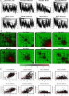
Figure 1
Figure 1. This motivational example explores the pairwise absolute correlations aij = |cor(xi,xj)| among 498 genes in different mouse tissues.
The biological significance of this network is described in ,. Each figure panel contains 8 subfigures for different genders and tissue types (liver, adipose, brain, muscle). (A) An average linkage hierarchical cluster tree of the genes. (B) The corresponding heat maps, which color-code the absolute pairwise correlations aij: red and green in the heat map indicate high and low absolute correlation, respectively. The genes in the rows and columns of each heat map are sorted by the corresponding cluster tree. (C) The relationship between gene significance GS (y-axis) and connectivity (x-axis). The gene significance of the ith gene was defined as the absolute correlation between the ith gene expression profile and mouse body weight. The hub gene significance HGS (Equation 13) is defined as the slope of the red line, which results from a regression model without an intercept term.
Figure 2
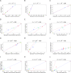
Figure 2. Relationships among maximum adjacency ratio, scaled connectivity, and gene significance.
(A) The relationship between MARi (y-axis) and scaled connectivity Ki using the female mouse muscle tissue network described in the motivational example. The genes are colored red or black depending on whether they are significantly (p-value<0.05) related to mouse body weight. (B) Boxplots and a Kruskal-Wallis test p-value (p = 0.00072) for studying whether MARi differs between significant (red) and non-significant (black) genes. (C) The analogous boxplots and p-value for the scaled connectivity Ki. In this female muscle tissue application, MARi is more significantly (p = 0.00072) related to GSi than is Ki (p = 0.051). (D,E,F) The analogous relationships for male muscle. Here, the MARi is more significantly (p = 0.00014) related to GSi than is Ki (p = 0.0034). (G,H,I) The analogous relationships for the brown module of the brain cancer application. Here, the MARi is slightly more significantly (p = 1.6E-8) related to GSi than is Ki (p = 2.6E-7). As a caveat, we mention that in other applications (e.g., the yeast network), we have found that Ki is more significantly related to GSi than MARi.
Figure 3
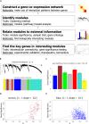
Figure 3. Overview and an example application of gene coexpression network analysis.
(A) Outline of an analysis flow chart. Gene coexpression network analysis aims to identify pathways (modules) and their key drivers (e.g., intramodular hub genes). (B) The hierarchical cluster tree of genes in the brain cancer network. Modules correspond to branches of the tree. The branches and module genes are assigned a color as can be seen from the color-bands underneath the tree. Grey denotes genes outside of proper modules. A functional enrichment analysis of these modules can be found in Horvath et al. (2006). (C) The module significance (average gene significance) of the modules. The underlying gene significance is defined with respect to the patient survival time (Equation 4). (D,E) Scatter plots of gene significance GS (y-axis) versus scaled connectivity K (x-axis) in the brown and blue module, respectively. The hub gene significance (Equation 13) is defined as the slope of the red line, which results from a regression model without an intercept term.
Figure 4
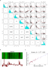
Figure 4. Module eigengenes in the brain cancer gene coexpression network.
(A) The pairwise scatter plots among the module eigengenes E (q) of different modules and cancer survival time T. Each dot represents a microarray sample. ME.blue denotes the module eigengene E (blue) of the blue module. Numbers below the diagonal are the absolute values of the corresponding correlations. Note that the module eigengenes of different modules can be highly correlated. The brown module eigengene has the highest absolute correlation (r = 0.20) with survival time. Frequency plots (histograms) of the variables are plotted along the diagonal. (B) Upper panel: heat map plot of the brown module gene expression profiles (rows) across the microarray samples (columns). Red corresponds to high- and green to low- expression values. Since the genes of a module are highly correlated, one observes vertical bands. (B) Lower panel: the values of the components of the module eigengene (y-axis) versus microarray sample number (x-axis). Note that vertical bands of red (green) in the upper panel correspond to high (low) values of the eigengene in the lower panel. (C) The expression profile of the module eigengene (y-axis) is highly correlated with that of the most highly connected hub gene (x-axis). A linear regression line has been added.
Figure 5
Figure 5. Using vectors to illustrate results in gene coexpression network analysis.
(A) A geometric interpretation of factorizability if the gene expression profiles and the module eigengene lie in a Euclidean plane. Then the angle θ 12 between gene expressions profiles 1 and 2 can be expressed in terms of angles with the module eigengene, i.e., θ 12 = θ 1θ 2. Similarly, θ 23 = θ 2+θ 3. Under the assumptions stated in the text, we find θij≈|θi±θj|. Using a trigonometric formula (Equation 51) this implies that the correlation matrix is approximately factorizable. (B) Illustrating why intramodular hub genes cannot be “intermediate” genes between two distinct coexpression modules. The large angle between module eigengenes E1 and E2 reflects that the corresponding modules are distinct. Since intermediate gene 1 does not have a small angle with either eigengene, it is not an intramodular hub gene. By contrast, intramodular hub gene 2 has a small angle with eigengene E1 but is not close to module eigengene E2. (C,D) Illustrating that the hub gene significance of a module depends on the relationship between the module eigengene and the underlying microarray sample trait (Equation 34). For sample traits T2 and T1 the hub gene significance (and corresponding eigengene significance cor(E,T)) are high and low, respectively. The geometry of (C) implies relationships between the connectivity k of a gene (determined by its angle with the eigengene E) and gene significance measure GS1 (its angle with trait T1) and GS2 (its angle with trait T2). As shown in (D), the gene significance measure GS2 increases with k since the small angle between E and T2 implies that genes with high k (small angle with E) also have a small angle with T2. In contrast, high connectivity k implies a large angle with T1 and thus GS1 decreases as a function of k.
Figure 6
Figure 6. Illustrating Observation 2 regarding the relationship between a network concept (y-axis) and its eigengene-based analog (x-axis) in the brain cancer data.
Each point corresponds to a module. (A–F) Corresponding to a weighted network constructed with a soft threshold (Equation 2) of β = 1. (G–L) Analogous plots for β = 6. (A,G) Centralization (y-axis) versus eigengene-based CentralizationE (x-axis). The following are analogous plots for (B,H): heterogeneity; (C,I) clustering coefficient; (D,J) module significance; and (E,K) hub gene significance. (F,L) Illustrating Equation 13 regarding the relationship between eigengene significance and hub gene significance. The blue line is the regression line through the points representing proper modules (i.e., the grey, nonmodule genes are left out). While the red reference line (slope 1, intercept 0) does not always fit well, we observe high squared correlations R 2 between network concepts and their analogs. Since the grey point corresponds to the genes outside properly defined modules, we did not include it in calculations.
Figure 7
Figure 7. Fuzzy module annotation of genes in the brain cancer network.
A natural choice for a fuzzy measure of module membership is the generalized scaled connectivity measure K cor,i (q) = |cor(xi,E (q))| (Equation 41). (A) Scatterplot of the brown module membership measure (y-axis) versus that of the blue module (x-axis). Note that grey dots corresponding to genes outside of properly defined modules can be intermediate between module genes. (B) The corresponding plot for blue versus turquoise module membership. (C) Brown versus turquoise module membership. (D) The relationship between gene significance based on survival time (y-axis) and brown module membership (x-axis).
Figure 8
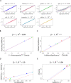
Figure 8. Using the brain cancer data to illustrate Observation 3 regarding the relationships among network concepts.
(A) Illustrating Equation 33 regarding the relationship between scaled intramodular connectivity Ki (q) (y-axis) and eigengene conformity ae ,i (x-axis). Each dot corresponds to a gene colored by its module membership. We find a high squared correlation R 2 even for the grey genes outside properly defined modules. (B) Illustrating Equation 31 regarding the relationship between the clustering coefficient and (1+Heterogeneity 2)2×Density. Again each dot represents a gene. The clustering coefficients of grey genes vary more than those of genes in proper modules. The short horizontal lines correspond to the mean clustering coefficient of each module. (C) Illustrating formula image (Equation 37); here each dot corresponds to a module. Since the grey dot corresponds to genes outside of properly defined modules, we have excluded it from the calculation of the squared correlation R 2. (D) Illustrating formula image (Equation 40); (E) Illustrating formula image (Equation 38). A reference line (red) with intercept 0 and slope 1 has been added to each plot. The blue line is the regression line through the points representing proper modules (i.e., the grey, non-module genes are left out). A robustness analysis with regard to different network construction methods, e.g., β>1, can be found in Text S1.
Figure 9
Figure 9. Using three different data (brain cancer, mouse liver, and yeast cell cycle) and three different network construction methods to illustrate Equation 37 regarding the relationship between module significance (y-axis) and (x-axis).
Points correspond to modules. The square of the correlation coefficient R 2 was computed without the grey, improper module. (A,D,G) Corresponding to the brain cancer gene coexpression networks. (B,E,H) Corresponding to mouse liver networks. (C,F,I) Corresponding to yeast networks. (A–C) Corresponding to a weighted network (Equation 2) constructed with soft thresholds β = 1. (D–F) Corresponding to β = 6. (G–I) Corresponding to an unweighted network (Equation 1) that results from thresholding the correlation matrix at τ = 0.5. Overall, we find that the reported relationship is quite robust with respect to our theoretical assumptions (e.g., factorizability). The blue line is the regression line through the points representing proper modules (i.e., the grey, nonmodule genes are left out). A reference line with slope 1 and intercept 0 is shown in red. Additional details can be found in Text S1, Text S2, and Text S3.

Similar articles

Cited by

References

    1. Ravasz E, Somera AL, Mongru DA, Oltvai ZN, Barabasi AL. Hierarchical organization of modularity in metabolic networks. Science. 2002;297:1551–1555. - PubMed
    1. Ihmels J, Bergmann S, Barkai N. Defining transcription modules using large-scale gene expression data. Bioinformatics. 2004;20:1993–2003. - PubMed
    1. Barabasi AL, Oltvai ZN. Network biology: understanding the cell's functional organization. Nat Rev Genet. 2004;5:101–113. - PubMed
    1. Albert R. Scale-free networks in cell biology. J Cell Sci. 2005;118:4947–4957. - PubMed
    1. Milo R, Shen-Orr S, Itzkovitz S, Kashtan N, Chklovskii D, et al. Network motifs: simple building blocks of complex networks. Science. 2002;298:824–827. - PubMed

Publication types