. 2008 Jul 23;28(30):7520-36.
doi: 10.1523/JNEUROSCI.0623-08.2008.

Highly selective receptive fields in mouse visual cortex

Affiliations

Highly selective receptive fields in mouse visual cortex

Cristopher M Niell et al. J Neurosci. .

Abstract

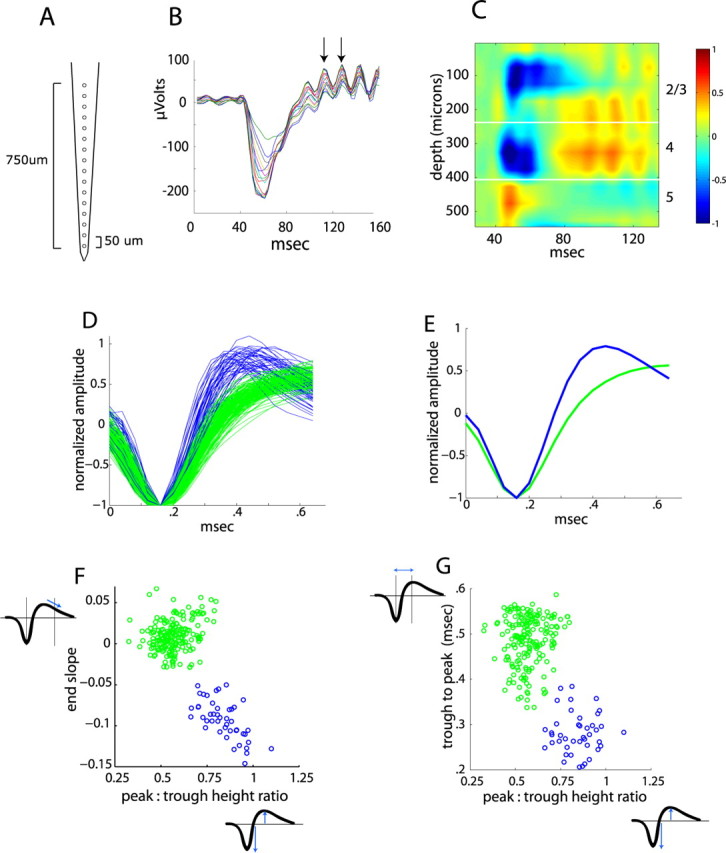
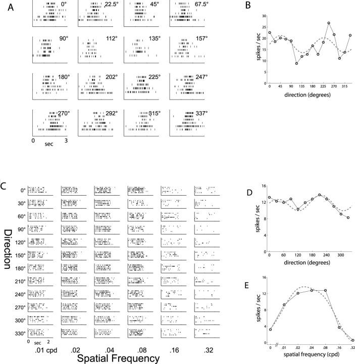
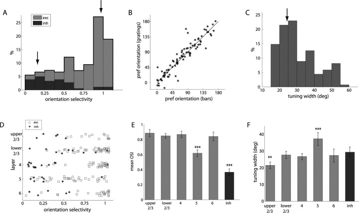
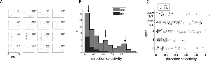
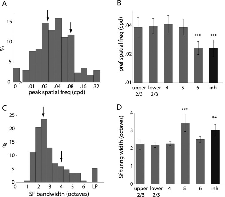
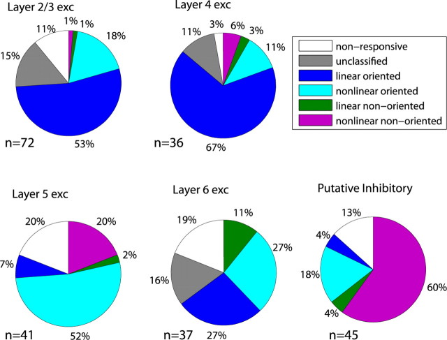
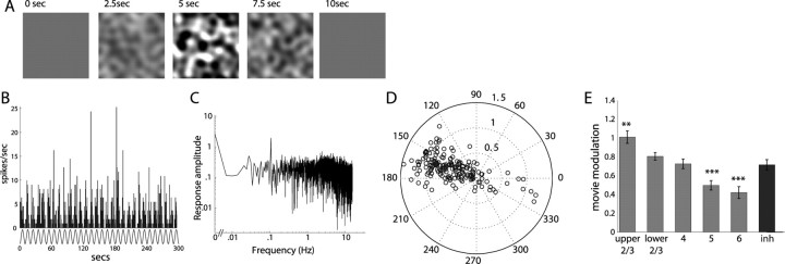
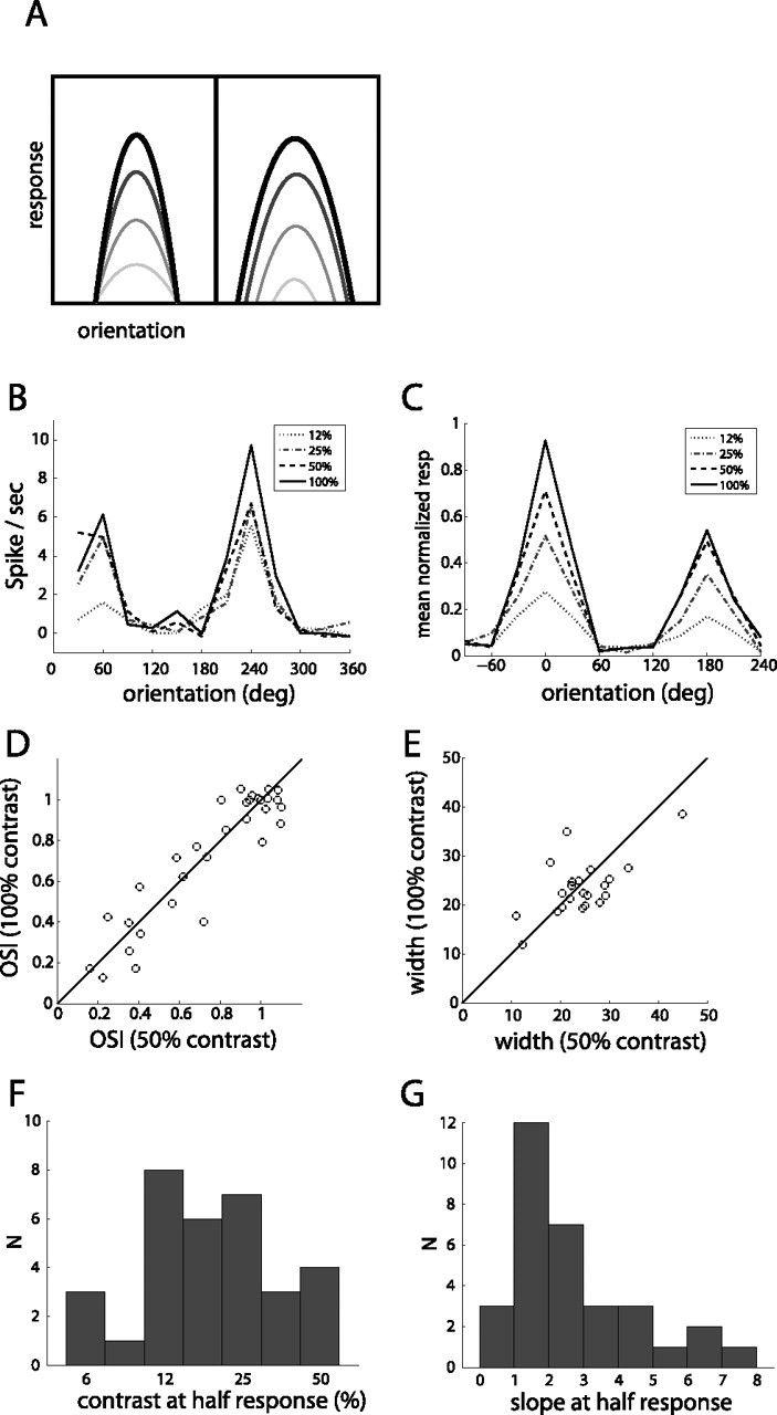
Genetic methods available in mice are likely to be powerful tools in dissecting cortical circuits. However, the visual cortex, in which sensory coding has been most thoroughly studied in other species, has essentially been neglected in mice perhaps because of their poor spatial acuity and the lack of columnar organization such as orientation maps. We have now applied quantitative methods to characterize visual receptive fields in mouse primary visual cortex V1 by making extracellular recordings with silicon electrode arrays in anesthetized mice. We used current source density analysis to determine laminar location and spike waveforms to discriminate putative excitatory and inhibitory units. We find that, although the spatial scale of mouse receptive fields is up to one or two orders of magnitude larger, neurons show selectivity for stimulus parameters such as orientation and spatial frequency that is near to that found in other species. Furthermore, typical response properties such as linear versus nonlinear spatial summation (i.e., simple and complex cells) and contrast-invariant tuning are also present in mouse V1 and correlate with laminar position and cell type. Interestingly, we find that putative inhibitory neurons generally have less selective, and nonlinear, responses. This quantitative description of receptive field properties should facilitate the use of mouse visual cortex as a system to address longstanding questions of visual neuroscience and cortical processing.


Figures

Figure 1.
Figure 1.
Laminar location and spike waveform classification. A, Schematic of linear multisite probe. B, Average LFP responses for 16 sites through the depth of cortex. Arrows show consecutive peaks of the high-frequency oscillation. C, CSD analysis of traces in B demonstrates segregation of responses by layer. Blue represents current sinks, and red represents current sources. Because the CSD is based on a second derivative at two-site spacing, the CSD cannot be computed for the top two and bottom two sites, so it spans 550 μm rather than 750 μm. Units for CSD are normalized from −1 to 1. D, Average spike waveforms for all units analyzed, aligned to minimum and normalized by trough depth, demonstrating narrow-spiking (blue; n = 45) and broad-spiking (green; n = 186) units. E, Average of all waveforms for narrow-spiking and broad-spiking units. F, G, Scatter plot of spike waveform parameters for all units.
Figure 2.
Figure 2.
Response properties of a typical oriented, linear unit. A, Spike rasters in response to drifting bars in 16 directions. B, Orientation tuning curve from rasters in A demonstrates sharp tuning. Dashed curve is fit to a sum of Gaussians. C, Spike rasters in response to drifting gratings of 12 directions and six spatial frequencies. Periodic response is indicative of a linear response type. D, Orientation tuning curve from rasters in C. E, Spatial frequency tuning curve shows bandpass selectivity. Dashed curve is fit to difference of Gaussians.
Figure 3.
Figure 3.
Response of a poorly selective, nonlinear putative inhibitory unit. A, Response to drifting bars of various orientations demonstrates minimal orientation selectivity. B, Orientation tuning curve from rasters in A, with fit to sum of Gaussians (dashed line). C, Response to drifting gratings shows continuous, rather than periodic, response, with minimal orientation tuning. D, Orientation tuning curve for drifting gratings. E, Spatial frequency tuning curve, with fit to difference of Gaussians (dashed line).
Figure 4.
Figure 4.
Orientation selectivity. A, Histogram of OSI for all responsive units (n = 182), with gray and black representing proportion of putative excitatory (exc) and inhibitory (inh) units. Arrows show values for units in Figures 2 and 3. B, Comparison of preferred orientation angle (degree) as measured with bars and gratings demonstrates consistency. C, Histogram of mean tuning width for all orientation-selective units (n = 135). Arrow shows value for unit in Figure 2. D, Orientation selectivity by layer and cell type. E, Mean OSI for each layer and cell type. F, Median width of orientation tuning for all oriented units by layer.
Figure 5.
Figure 5.
Direction selectivity. A, Spike rasters for response of a representative direction-selective unit to bars drifting in 16 directions. B, Histogram of direction selectivity from drifting gratings across the population of recorded units (n = 182), with gray and black representing relative proportion of putative excitatory (exc) and inhibitory (inh) units. Arrows show values from units shown in Figures 3, 2, and 5 A, respectively. C, Distribution of direction selectivity by layer and cell type shows that most highly direction-selective cells are putative excitatory units in layers 2/3 and 4.
Figure 6.
Figure 6.
Spatial frequency tuning. A, Histogram of peak spatial frequency response. B, Median peak spatial frequency across layers demonstrates lower preferred spatial frequency in layer 6 and putative inhibitory (inh) units. C, Width of spatial frequency tuning. Arrows in A and C show values from units presented in Figures 2 and 3. LP, Low-pass tuning. D, Median spatial frequency tuning width shows broader tuning in layer 5 and putative inhibitory units. n = 182 units total; n = 14, 40, 31, 34, 24, and 39 by cell type.
Figure 7.
Figure 7.
Linearity of response to drifting gratings. A, Histogram of F 1/F 0 ratio across entire population (n = 182), with black and gray showing relative proportion of putative inhibitory (inh) and excitatory (exc) units. Arrows show units from Figures 3 and 2 (left and right, respectively). B, Distribution of linearity by layer and cell type. C, Fraction of units with linear responses (F 1/F 0 > 1).
Figure 8.
Figure 8.
Receptive field size, firing rates, and temporal frequency response. A, Receptive field size measured with small sweeping bars, segregated by layer and cell type. n = 108 units. B, Mean receptive field size of each group. C, Logarithmic plot of spontaneous firing rate for all units, by layer and cell type. n = 231 units. D, Median spontaneous firing rate of each group. E, Firing rate in response to optimal grating stimulus, for all visually responsive units (n = 204), averaged over 1.5 s presentation. [Instantaneous firing rates are shown in supplemental Fig. S3 (available at www.jneurosci.org as supplemental material).] F, Median response to optimal stimulus for each group. G, Median peak temporal frequency, averaged for layers and cell type, showing higher temporal frequency response in layer 4. n = 96 units. H, Mean temporal frequency tuning, comparing response in layers 2/3 and 4. exc, Putative excitatory units; inh, putative inhibitory units.
Figure 9.
Figure 9.
Distribution of functional response categories for layers and cell types. exc, Putative excitatory units.
Figure 10.
Figure 10.
Response to contrast-modulated noise movies. A, Frames from a contrast-modulated movie. B, Spike histogram in response to contrast-modulated movie, with movie contrast in gray below. C, Power spectrum of response, showing peak at fundamental frequency of contrast modulation (0.1 Hz). D, Polar plot of response modulation and phase at the fundamental frequency (n = 188). E, Histogram of response modulation with contrast, for different layers and cell types, shows decreased responsiveness in deeper layers. inh, Putative inhibitory units.
Figure 11.
Figure 11.
Receptive fields by spike-triggered average. A–C, Examples of spatial receptive fields with two, three, and one subfield, respectively, showing varying orientation, ON/OFF centers, and spacing of subfields. D, Comparison of preferred orientation from STA receptive fields versus orientation measured from gratings. E, Comparison of receptive field spatial frequency from STA versus gratings shows good correspondence for units with spatial frequency greater than 0.017 cpd (blue) and poor correspondence for units with the lowest spatial frequencies (gray). F, Median width of orientation tuning for units with differing numbers of subunits in the STA. G, Median bandwidth of spatial frequency tuning for varying number of subunits. H, Residual error in fit of STA to Gabor function. I, Geometric description of receptive field structure for units accurately fit by Gabors compared with macaque from Ringach (2002). J, Distribution of spatial phase in Gabor fits, in which 0° represents even symmetry and 90° represents odd symmetry.
Figure 12.
Figure 12.
Contrast-invariant tuning and contrast–response characteristics. A, Schematic of contrast-invariant (left) versus contrast-dependent (right) orientation tuning. B, Example of orientation tuning in response to gratings of different contrast, for unit in Figure 2. C, Orientation tuning at different contrasts averaged across 22 orientation-selective units. Tuning curves of each unit were aligned to preferred orientation and normalized to maximum response before averaging. D, Comparison of orientation selectivity at 50 and 100% contrast shows no systematic change (n = 32). E, Width of tuning, for orientation-selective units (n = 22), at 50 and 100% contrast. F, Value of contrast that gave half-maximal response (n = 32). G, Slope of the contrast response function at half-maximal response.

Similar articles

Cited by

References

    1. Andermann ML, Ritt J, Neimark MA, Moore CI. Neural correlates of vibrissa resonance; band-pass and somatotopic representation of high-frequency stimuli. Neuron. 2004;42:451–463. - PubMed
    1. Anderson JS, Carandini M, Ferster D. Orientation tuning of input conductance, excitation, and inhibition in cat primary visual cortex. J Neurophysiol. 2000;84:909–926. - PubMed
    1. Antonini A, Fagiolini M, Stryker MP. Anatomical correlates of functional plasticity in mouse visual cortex. J Neurosci. 1999;19:4388–4406. - PMC - PubMed
    1. Atencio CA, Schreiner CE. Spectrotemporal processing differences between auditory cortical fast-spiking and regular-spiking neurons. J Neurosci. 2008;28:3897–3910. - PMC - PubMed
    1. Barthó P, Hirase H, Monconduit L, Zugaro M, Harris KD, Buzsáki G. Characterization of neocortical principal cells and interneurons by network interactions and extracellular features. J Neurophysiol. 2004;92:600–608. - PubMed

Publication types

LinkOut - more resources