

Persistent cell motion in the absence of external signals: a search strategy for eukaryotic cells
- PMID: 18461173
- PMCID: PMC2358978
- DOI: 10.1371/journal.pone.0002093
Persistent cell motion in the absence of external signals: a search strategy for eukaryotic cells
Abstract
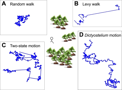
Background: Eukaryotic cells are large enough to detect signals and then orient to them by differentiating the signal strength across the length and breadth of the cell. Amoebae, fibroblasts, neutrophils and growth cones all behave in this way. Little is known however about cell motion and searching behavior in the absence of a signal. Is individual cell motion best characterized as a random walk? Do individual cells have a search strategy when they are beyond the range of the signal they would otherwise move toward? Here we ask if single, isolated, Dictyostelium and Polysphondylium amoebae bias their motion in the absence of external cues.
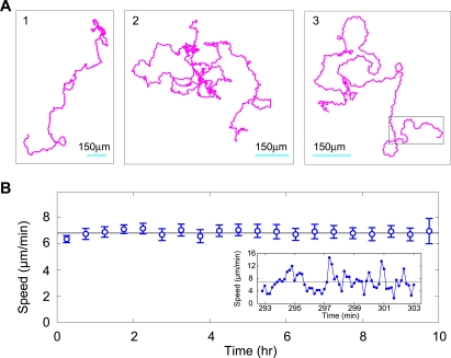
Methodology: We placed single well-isolated Dictyostelium and Polysphondylium cells on a nutrient-free agar surface and followed them at 10 sec intervals for approximately 10 hr, then analyzed their motion with respect to velocity, turning angle, persistence length, and persistence time, comparing the results to the expectation for a variety of different types of random motion.
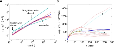
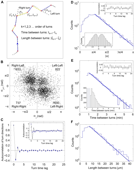
Conclusions: We find that amoeboid behavior is well described by a special kind of random motion: Amoebae show a long persistence time ( approximately 10 min) beyond which they start to lose their direction; they move forward in a zig-zag manner; and they make turns every 1-2 min on average. They bias their motion by remembering the last turn and turning away from it. Interpreting the motion as consisting of runs and turns, the duration of a run and the amplitude of a turn are both found to be exponentially distributed. We show that this behavior greatly improves their chances of finding a target relative to performing a random walk. We believe that other eukaryotic cells may employ a strategy similar to Dictyostelium when seeking conditions or signal sources not yet within range of their detection system.
Conflict of interest statement
Figures
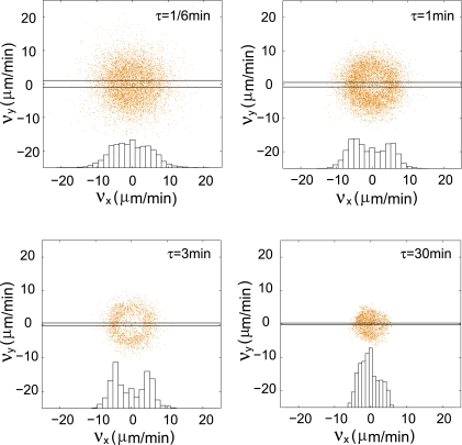
 and vx was plotted vs vy with increasing τ. Larger and larger gaps at the centers of the distributions with time demonstrate that the cell velocity distributions are non-Gaussian. As expected, at very large τ, the distribution approaches a Gaussian again. Inserts, histograms of the x component of the velocities for the intervals defined by the parallel lines.
Similar articles
-
Zigzag turning preference of freely crawling cells.PLoS One. 2011;6(6):e20255. doi: 10.1371/journal.pone.0020255. Epub 2011 Jun 7. PLoS One. 2011. PMID: 21687729 Free PMC article.
-
Food searching strategy of amoeboid cells by starvation induced run length extension.PLoS One. 2009 Aug 28;4(8):e6814. doi: 10.1371/journal.pone.0006814. PLoS One. 2009. PMID: 19714242 Free PMC article.
-
Quantifying the degree of persistence in random amoeboid motion based on the Hurst exponent of fractional Brownian motion.Phys Rev E Stat Nonlin Soft Matter Phys. 2014 Oct;90(4):042703. doi: 10.1103/PhysRevE.90.042703. Epub 2014 Oct 6. Phys Rev E Stat Nonlin Soft Matter Phys. 2014. PMID: 25375519
-
Mechanisms of gradient detection: a comparison of axon pathfinding with eukaryotic cell migration.Int Rev Cytol. 2007;263:1-62. doi: 10.1016/S0074-7696(07)63001-0. Int Rev Cytol. 2007. PMID: 17725964 Review.
-
Mechanisms of excitation and adaptation in Dictyostelium.Semin Cell Biol. 1990 Apr;1(2):99-104. Semin Cell Biol. 1990. PMID: 2129339 Review.
Cited by
-
A Fully Integrated Arduino-Based System for the Application of Stretching Stimuli to Living Cells and Their Time-Lapse Observation: A Do-It-Yourself Biology Approach.Ann Biomed Eng. 2021 Sep;49(9):2243-2259. doi: 10.1007/s10439-021-02758-3. Epub 2021 Mar 16. Ann Biomed Eng. 2021. PMID: 33728867
-
Excitable behavior in amoeboid chemotaxis.Wiley Interdiscip Rev Syst Biol Med. 2013 Sep-Oct;5(5):631-42. doi: 10.1002/wsbm.1230. Epub 2013 Jun 11. Wiley Interdiscip Rev Syst Biol Med. 2013. PMID: 23757165 Free PMC article. Review.
-
Theoretical model for cell migration with gradient sensing and shape deformation.Eur Phys J E Soft Matter. 2013 Apr;36(4):9846. doi: 10.1140/epje/i2013-13032-1. Epub 2013 Apr 11. Eur Phys J E Soft Matter. 2013. PMID: 23572335
-
A Novel Method for Effective Cell Segmentation and Tracking in Phase Contrast Microscopic Images.Sensors (Basel). 2021 May 18;21(10):3516. doi: 10.3390/s21103516. Sensors (Basel). 2021. PMID: 34070081 Free PMC article.
-
Elements of the cellular metabolic structure.Front Mol Biosci. 2015 Apr 28;2:16. doi: 10.3389/fmolb.2015.00016. eCollection 2015. Front Mol Biosci. 2015. PMID: 25988183 Free PMC article.
References
-
- Viswanathan GM, Buldyrev SV, Havlin S, da Luz MG, Raposo EP, et al. Optimizing the success of random searches. Nature. 1999;401:911–914. - PubMed
-
- Bartumeus F, Catalan J, Fulco UL, Lyra ML, Viswanathan GM. Optimizing the encounter rate in biological interactions: Levy versus Brownian strategies. Phys Rev Lett. 2002;88:097901. - PubMed
-
- Raposo EP, Buldyrev SV, da Luz MGE, Santos MC, Stanley HE, et al. Dynamical robustness of Levy search strategies. Phys Rev Lett. 2003;91:240601. - PubMed
-
- Santos MC, Viswanathan GM, Raposo EP, da Luz MGE. Optimization of random searches on regular lattices. Phys Rev E. 2005;72:046143. - PubMed
-
- Edwards AM, Phillips RA, Watkins NW, Freeman MP, Murphy EJ, et al. Revisiting Levy flight search patterns of wandering albatrosses, bumblebees and deer. Nature. 2007;449:1044–1048. - PubMed
Publication types
MeSH terms
Grants and funding
LinkOut - more resources
Full Text Sources
Miscellaneous
