. 2024 Oct 2:23:3537-3548.
doi: 10.1016/j.csbj.2024.09.025. eCollection 2024 Dec.

Multiscale molecular modeling of chromatin with MultiMM: From nucleosomes to the whole genome

Affiliations

Multiscale molecular modeling of chromatin with MultiMM: From nucleosomes to the whole genome

Sevastianos Korsak et al. Comput Struct Biotechnol J. .

Abstract

Motivation: We present a user-friendly 3D chromatin simulation model for the human genome based on OpenMM, addressing the challenges posed by existing models with use-specific implementations. Our approach employs a multi-scale energy minimization strategy, capturing chromatin's hierarchical structure. Initiating with a Hilbert curve-based structure, users can input files specifying nucleosome positioning, loops, compartments, or subcompartments. Results: The model utilizes an energy minimization approach with a large choice of numerical integrators, providing the entire genome's structure within minutes. Output files include the generated structures for each chromosome, offering a versatile and accessible tool for chromatin simulation in bioinformatics studies. Furthermore, MultiMM is capable of producing nucleosome-resolution structures by making simplistic geometric assumptions about the structure and the density of nucleosomes on the DNA. Code availability: Open-source software and the manual are freely available on https://github.com/SFGLab/MultiMM or via pip https://pypi.org/project/MultiMM/.


Conflict of interest statement

Authors do not acknowledge any conflicts of interest.

Figures

None
Graphical abstract
Fig. 1
Fig. 1
Flowchart of MultiMM. The process begins with the user selecting a 3C-type experiment and extracting loop and (sub)compartment interactions. MultiMM then takes these data as input and converts them into simulation quantities through unit rescaling. These quantities are imported into the OpenMM force field and applied to an initially generated Hilbert curve structure. After a period of simulation, the final genome-wide structures are produced. If ATAC-Seq data is provided, MultiMM can also generate structures inclusive of nucleosomes.
Fig. 2
Fig. 2
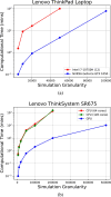
Benchmarking of MultiMM based on computational time: (a) performed on a Lenovo ThinkPad laptop and (b) on a Lenovo Hopper server. The y-axis represents computational time in minutes (logarithmic scale), while the x-axis corresponds to varying values of simulation granularity, Nbeads. In subfigure (b), the server allows simulations of one order of magnitude larger than those achievable on the ThinkPad.
Fig. 3
Fig. 3
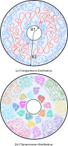
The location of compartments and chromosomes in the genome. (a) Compartments are localized in such a way that they are attracted by the outer and inner lamina. (b) Chromosomes are localized so that smaller chromosomes are closer to the center, whereas bigger ones are localized in the outer regions.
Fig. 4
Fig. 4
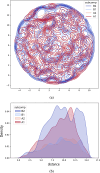
Direct validation of lamina function and compartmentalization interactions. (a) 2D spartial distribution of compartmentalization. The B compartment, which is attracted to the lamina, is concentrated near the nuclear periphery, whereas the A compartment is concentrated in the intermediate region between the inner and outer laminas. (b) The radial distribution of subcompartments demonstrates that the B compartment is attracted to the inner lamina as well and exhibits a bimodal distribution.
Fig. 5
Fig. 5
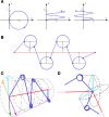
Nucleosome interpolation scheme. (A) Three orthogonal projections of the generic helix which serve as a nucleosome model. Here, helix makes 1.65 turns. r and h denote the nucleosome radius and height respectively. (B) Positioning of the consecutive nucleosome along the original chromatin fragment (red segment). Here, r and L denote nucleosome radius and half of the linker length. Linker length may be constant or is variable in the “random” mode of the simulation. The chromatin interpolated with nucleosomes depicted in blue. (C) The rotation of consecutive nucleosome positioning in “zigzag” configuration. The red segment represents the chromatin fragment. The position of the fist nucleosome is determined by the first “zigzag” vector (cyan). Second vector (green) is rotated 180. Third vector (orange) is rotated 180 + ϕnorm and the fourth (pink) another 180. In “random” configuration the angles are randomized. (D) Junction between chromatin fragments (red segments). The last “zigzag” vector is projected onto the plane orthogonal to the next chromatin fragment and reversed. This procedure ensured relative continuity of the zigzag pattern when crossing between chromatin fragments.
Fig. 6
Fig. 6
Changes in chromatin structure resulting from variations in hyper-parameters for chromosomal block strength, central force strength, and B-lamina interaction strength. Each structure comprises 50,000 beads. The parameter values are: (A) chromosomal block strength: 10−4, 10−3, 10−2, 10−1 kJ/mol; (B) central force strength: 10, 100, 500, 1000 kJ/mol; and (C) B-lamina interaction strength: 100, 400, 1000, 5000 kJ/mol.
Fig. 7
Fig. 7
Results from modeling with MultiMM. (A) Visualization of different chromatin scales using PyVista . (B) The upper graph displays a plot comparing individual simulated and random inverse-distance heatmaps with corresponding experimental data. The lower graph presents a similar comparison, showcasing averages over multiple samples of heatmaps correlated with experimental data. Each structure consisted of 10,000 beads. (C) Pearson correlation coefficients between the heatmaps of structures modeled with 1,000 beads across 1,000 random 20 Mb regions of chromatin, compared to the experimental data.
Fig. 8
Fig. 8
Comparison between modeling with population averaged and single cell data as input. The granularity of MultiMM whole genome structure in these simulations is 100000 beads with the default parameters as input.

Similar articles

References

    1. Zhou R., Gao Y.Q. Polymer models for the mechanisms of chromatin 3d folding: review and perspective. Phys Chem Chem Phys. 2020;22:20189–20201. doi: 10.1039/D0CP01877E. - DOI - PubMed
    1. Sikorska N., Sexton T. Defining functionally relevant spatial chromatin domains: it is a tad complicated. J Mol Biol. 12.2019;432(12) doi: 10.1016/j.jmb.2019.12.006. - DOI - PubMed
    1. Ea V., Baudement M.-O., Lesne A., Forné T. Contribution of topological domains and loop formation to 3d chromatin organization. Genes. 2015;6(3):734–750. - PMC - PubMed
    1. Bianco S., Chiariello A.M., Annunziatella C., Esposito A., Nicodemi M. Predicting chromatin architecture from models of polymer physics. Chromosom Res. 2017;25:25–34. - PubMed
    1. Biswas M., Langowski J., Bishop T.C. Atomistic simulations of nucleosomes. Wiley Interdiscip Rev Comput Mol Sci. 2013;3(4):378–392.

LinkOut - more resources