. 2024 Aug 20;15(1):7136.
doi: 10.1038/s41467-024-51433-3.

An end-to-end deep learning method for mass spectrometry data analysis to reveal disease-specific metabolic profiles

Affiliations

An end-to-end deep learning method for mass spectrometry data analysis to reveal disease-specific metabolic profiles

Yongjie Deng et al. Nat Commun. .

Abstract

Untargeted metabolomic analysis using mass spectrometry provides comprehensive metabolic profiling, but its medical application faces challenges of complex data processing, high inter-batch variability, and unidentified metabolites. Here, we present DeepMSProfiler, an explainable deep-learning-based method, enabling end-to-end analysis on raw metabolic signals with output of high accuracy and reliability. Using cross-hospital 859 human serum samples from lung adenocarcinoma, benign lung nodules, and healthy individuals, DeepMSProfiler successfully differentiates the metabolomic profiles of different groups (AUC 0.99) and detects early-stage lung adenocarcinoma (accuracy 0.961). Model flow and ablation experiments demonstrate that DeepMSProfiler overcomes inter-hospital variability and effects of unknown metabolites signals. Our ensemble strategy removes background-category phenomena in multi-classification deep-learning models, and the novel interpretability enables direct access to disease-related metabolite-protein networks. Further applying to lipid metabolomic data unveils correlations of important metabolites and proteins. Overall, DeepMSProfiler offers a straightforward and reliable method for disease diagnosis and mechanism discovery, enhancing its broad applicability.


Conflict of interest statement

All authors declare the following competing interests. All authors have filed patents for both the technology and the use of the technology to analyse metabolomic data.

Figures
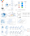
Fig. 1
Fig. 1. The DeepMSProfiler method using LC-MS-based untargeted serum metabolome.
a The overview of DeepMSProfiler. Serum samples of different populations (top left) were collected and sent to the instrument (bottom left) for liquid chromatography-mass spectrometry (LC-MS) analysis. The raw LC-MS data, containing information on retention time (RT), mass-to-charge ratio (m/z), and intensity, is used as input to the ensemble model (middle). Multiple single convolutional neural networks form the ensemble model (centre) to predict the true label of the input data and generate three outputs (right), including the predicted sample classes, the contribution heatmaps of classification-specific metabolic signals, and the classification-specific metabolic networks. b The data structure of raw data. The mass spectra of different colours (centre) represent the corresponding m/z and ion intensity of ion signal groups recorded at different RT frames. All sample points are distributed in a three-dimensional space (left) which can be mapped along three axes to obtain chromatograms, mass spectra, and two-dimensional matrix data. Chromatograms and mass spectra are used for conventional qualitative and quantitative analysis (right), while the two-dimensional matrix serves as input data for convolutional neural networks. c The structure of a single end-to-end model. The input data undergoes the pre-pooling processing to reduce dimensionality and become three-channel data. As the model passes through each convolutional layer (conv) in the feature extractor module, the weights associated with the original signals change continuously. The sizes of different frames in the enlarged layers (top) represent different receptive fields, with DenseNet allowing the model to generate more flexible receptive field sizes. After the last fully connected layer (FC), the classifications are resulted.
Fig. 2
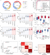
Fig. 2. The prediction performance of DeepMSProfiler.
a The sample allocation chart. The outer ring indicates the types of diseases and the inner ring indicates the sex distribution. Healthy: healthy individuals; Benign: benign lung nodules; Malignant: lung adenocarcinoma. b Predicted receiver operating characteristic (ROC) curves of different methods. Random: performance baseline in a random state. Comparison of performance metrics of different methods (n = 50): accuracy (c), precision (d), recall (e), and F1 score (f). The blue areas show the different conventional analysis processes using machine learning methods, and the red areas display different end-to-end analysis processes using deep learning methods. The boxplot shows the minimum, first quartile, median, third quartile and maximum values, with outliers as outliers. g Model accuracy rates for different age groups. The sample sizes for different groups are 52, 69, 40, and 12, respectively. h Model accuracy rates for different lesion diameter groups. The sample sizes for different groups are 27, 37, 18, 13, and 34, respectively. The boxplot shows the minimum, first quartile, median, third quartile and maximum values. i Prediction accuracy and parameter scale of different model architectures. j The confusion matrix of the DeepMSProfiler model. The numbers inside the boxes are the number of matched samples between the true label and the predicted label. The ratio in parentheses is the number of matched samples divided by the number of all samples of the true label.
Fig. 3
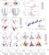
Fig. 3. Explainable deep learning method avoids limitations of batch effects in conventional methods.
a Batch effects in 3D point array and 2D mapped heatmap of reference samples. RT: retention time; m/z: mass-to-charge ratio. b Isotope peaks of the same concentration in different samples. Different colours represent the batches to which the samples belong. c The visualisation of dimensionality reduction of normalisation by the Reference Material method. Below: different colours represent different classes; Above: different colours indicate different batches. Healthy: healthy individuals; Benign: benign lung nodules; Malignant: lung adenocarcinoma. d The visualisation of dimensionality reduction for the output data of the hidden layers in DeepMSProfiler. Conv1 to Conv5 are the outputs of the first to the fifth pooling layer in the feature extraction module. Block4 and Block5 are the outputs of the fourth and fifth conv layers in the fifth feature extraction module. Upper: different colours indicate different sample batches; Lower: different colours represent different population classes. e Correlation of the output data of the hidden layer with the batch and class information in DeepMSProfiler. The horizontal axis represents the layer names. Conv1 to Conv5 are the outputs of the first to the fifth pooling layer in the feature extraction module. Block10 and Block16 are the outputs of the tenth and sixteenth conv layers in the fifth feature extraction module. The blue line represents the batch-related correlations, and the orange line illustrates the classification-related correlations. f The accuracy rates of traditional methods (blue), corrected methods based on reference samples (purple), and DeepMSProfiler (red) in independent testing dataset (n = 50). The boxplot shows the minimum, first quartile, median, third quartile and maximum values, with outliers as outliers.
Fig. 4
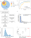
Fig. 4. The unknown space in databases and previous studies.
a Statistics of annotated metabolite peaks. Blue colour represents all peaks, orange, purple and while yellow colours indicate metabolites annotated in HMDB, KEGG, and all databases, respectively. The overlap between orange and purple includes 414 metabolites annotated in both HMDB and KEGG. HMDB: Human Metabolome Database; KEGG: Kyoto Encyclopedia of Genes and Genomes. b The feature selection plot illustrates the effect of different contribution score thresholds removing unknown metabolites versus non-removing. The horizontal axis represents the change in threshold, while the vertical axis shows the accuracy of the model using the remaining features. The shadings of solid lines (mean) represent error bars (standard deviation). c Collection standard of published lung cancer serum metabolic biomarker. SCLC: Small Cell Lung Cancer; LUSC: Lung Squamous Cell Carcinoma; LUAD: Lung Adenocarcinoma; NAR: Nuclear Magnetic Resonance; MS: Mass Spectrometry. d The number counts of known biomarkers published in the current literature. e Molecular weight distribution plot of known biomarkers. f Accuracy comparison between the ablation experiment and DeepMSProfile (n = 50). The boxplot shows the minimum, first quartile, median, third quartile and maximum values. In the ablation experiment, we investigated the effect of varying the publication count (PC) of known biomarkers in the literature. Specifically, we eliminated metabolic signals that were not reported in the original data based on the m/z of known biomarkers. We retained only the metabolic signals with publication counts greater than 1, greater than 3, and greater than 8 for modelling development. All ablated data was analysed using the same architecture as the original unprocessed data in the same DeepMSProfiler architecture. The vertical axis shows the accuracy of models built on the dataset of different publication counts and our DeepMSProfiler.
Fig. 5
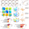
Fig. 5. Feature constructions of prediction and significant metabolic signals relevant to biological pathways.
a Prediction performance and feature scoring by different single models. b Prediction performance and feature scoring by DeepMSProfiler. c Heatmap matrices of classification contribution in healthy individuals (Healthy), benign lung nodules (Benign), and lung adenocarcinoma (Malignant). The horizontal and vertical axes of the matrix are the prediction label and the true label, respectively. The heatmaps of upper left, the middle one, and the bottom right represent the true healthy individuals, the true benign nodules, and the true lung adenocarcinoma, respectively. The horizontal and vertical axes of each heatmap are RT and m/z, respectively. The classification contributions of metabolites corresponding to true healthy individuals (d), benign nodules (e), and lung adenocarcinoma (f). The horizontal axis represents the retention time and the vertical axis represents the m/z of the corresponding metabolites. The colours represent the contribution score of the metabolites. The redder the colour, the greater the contribution to the classification. Metabolites-proteins network for healthy individuals (g), benign nodules (h), and lung adenocarcinoma (i). Pathway enrichment analysis using the signalling networks for healthy individuals (j), benign nodules (k), and lung adenocarcinoma (l) (FDR < 0.05). m/z: mass charge ratio, RT: retention time.
Fig. 6
Fig. 6. Metabolite and protein associations across 23 cancer types.
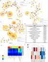
Metabolite-protein networks for (a) lung cancer, (b) gastric cancer, and (c) leukaemia. Yellow squares: metabolites. Red circles: proteins. Blue labels: metabolites and proteins shared in 23 cancer metabolite-protein networks. d Metabolites and proteins shared in the metabolite-protein networks of 23 cancer types. e Heatmap of the classification contribution of different lipid metabolites across 23 cancer types. f Correlation of important pan-cancer-related metabolites with methylation of the PLA and UGT gene families.

Similar articles

References

    1. Schmidt, D. R. et al. Metabolomics in cancer research and emerging applications in clinical oncology. CA Cancer J. Clin.71, 333–358 (2021). 10.3322/caac.21670 - DOI - PMC - PubMed
    1. Li, H. et al. The landscape of cancer cell line metabolism. Nat. Med.25, 850–860 (2019). 10.1038/s41591-019-0404-8 - DOI - PMC - PubMed
    1. Buergel, T. et al. Metabolomic profiles predict individual multidisease outcomes. Nat. Med.28, 2309–2320 (2022). 10.1038/s41591-022-01980-3 - DOI - PMC - PubMed
    1. Yang, J., Huang, L. & Qian, K. Nanomaterials‐assisted metabolic analysis toward in vitro diagnostics. Exploration2, 20210222 (2022). - PMC - PubMed
    1. Marx, V. Boost that metabolomic confidence. Nat. Methods17, 33–36 (2020). 10.1038/s41592-019-0694-2 - DOI - PubMed

LinkOut - more resources