. 2024 Jul 9;6(3):lqae082.
doi: 10.1093/nargab/lqae082. eCollection 2024 Sep.

Data-driven probabilistic definition of the low energy conformational states of protein residues

Affiliations

Data-driven probabilistic definition of the low energy conformational states of protein residues

Jose Gavalda-Garcia et al. NAR Genom Bioinform. .

Abstract

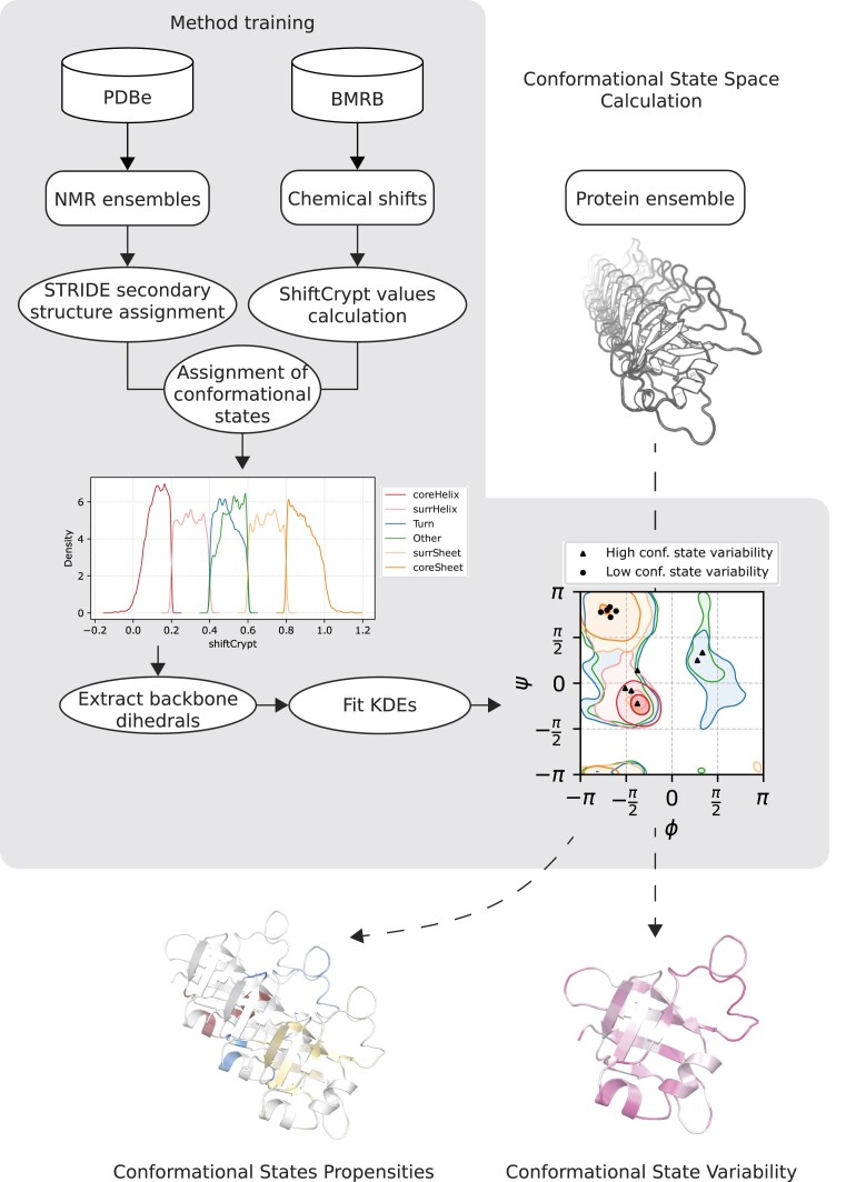
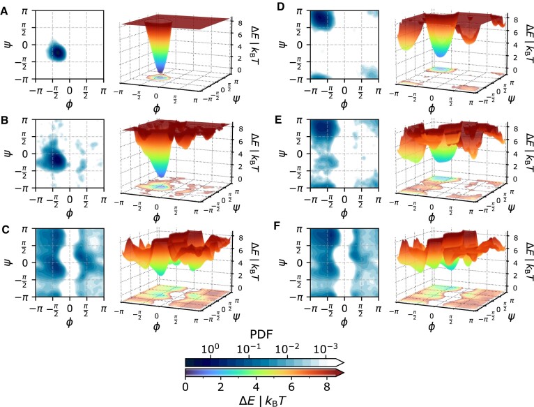
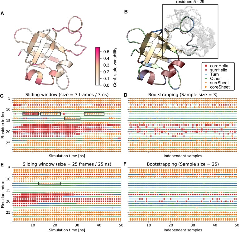
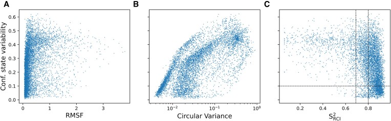
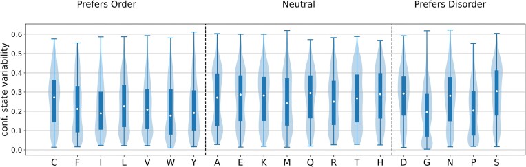
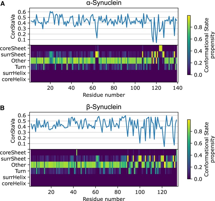
Protein dynamics and related conformational changes are essential for their function but difficult to characterise and interpret. Amino acids in a protein behave according to their local energy landscape, which is determined by their local structural context and environmental conditions. The lowest energy state for a given residue can correspond to sharply defined conformations, e.g. in a stable helix, or can cover a wide range of conformations, e.g. in intrinsically disordered regions. A good definition of such low energy states is therefore important to describe the behaviour of a residue and how it changes with its environment. We propose a data-driven probabilistic definition of six low energy conformational states typically accessible for amino acid residues in proteins. This definition is based on solution NMR information of 1322 proteins through a combined analysis of structure ensembles with interpreted chemical shifts. We further introduce a conformational state variability parameter that captures, based on an ensemble of protein structures from molecular dynamics or other methods, how often a residue moves between these conformational states. The approach enables a different perspective on the local conformational behaviour of proteins that is complementary to their static interpretation from single structure models.


Conflict of interest statement

None declared.

Figures

Graphical Abstract
Graphical Abstract
Figure 1.
Figure 1.
Visual representation of the KDE training workflow and the calculation of conformational state propensities and conformational state variability. The training of the models (grey background region) employs NMR ensembles from the PDBe and chemical shift information from the BMRB. The NMR ensembles are used to obtain secondary structure assignments of each residue. The chemical shifts are employed to calculate the ShiftCrypt values. Both data sources are combined to assign the residues to a conformational state. Once the conformational state assignment of these residues is completed, their backbone dihedrals are extracted and used to fit six KDEs, one per conformational state. With these trained KDEs the conformational states probabilities as well as the conformational state variability can be calculated (dashed arrows).
Figure 2.
Figure 2.
Definition of the six conformational states in (ϕ, ψ)-space. Each panel shows a conformational state represented by a continuous probability density function on the left, and the derived potential energy surfaces in the (ϕ, ψ)-space on the right. The conformational states are shown for: (A) Core helix, (B) Surrounding helix, (C) Turn, (D) Core sheet, (E) Surrounding sheet and (F) Other. The potential energy surfaces illustrate how, e.g. a Core helix residue is conformationally restricted by high energy barriers, while Turn residues can adopt a wide range of backbone conformations without having to overcome such high energy barriers. This is further exemplified by the 2D projection in Supplementary Figure S12.
Figure 3.
Figure 3.
Analysis of MD simulation ensembles with Constava. The method was applied on the conformational ensemble derived from 100 ns of MD simulation on E. coli ribosomal protein L25 (PDB ID: 1b75). (A) Conformational state variability mapped on the structure. Regions of high variability are the loop region as well as the C-terminal end of the helical region, which switches between helical and turn-like states. (B) Conformational states propensities mapped on the structure. The rectangle highlights residues 5–29, where the largest conformational changes occur. (C) Conformational states as a time series along the simulation, using a sliding window with N = 3 (here 3 ns). Black boxes highlight transient conformational states apparent at this time-resolution. (D) Conformational states obtained from bootstrapping (N = 3). Adjacent samples are not related. Transient states are sometimes detected, but are underrepresented in comparison to the sliding-window method. (E) Conformational states as a time series along the simulation, using a sliding window with N = 25 (here 25 ns). Black boxes highlight transient conformational states apparent at this time-resolution. Notably, fewer transient states are detected compared to the smaller window size (panel C). (F) Conformational states obtained from bootstrapping (N = 25). With increasing sample size the likelihood to detect low populated transient conformational states further diminishes, and the detected conformational states increasingly converge on unique solutions.
Figure 4.
Figure 4.
Comparison of conformational state propensities with traditional secondary structure assignments. The plot shows residues 60–130 of Endonuclease V (PDB ID: 2end). (A) Assignments of Core helix propensities for the first 300 ns of the simulation. Notably, Constava continuously detects Core helix propensities ∼0.6 for residues 95–100. (B) DSSP assignment of H (α-helix) for the first 300 ns of the simulation. As DSSP performs a classification, the propensities for H are 0 or 1. The transient helix for residues 95–100 only appears shortly after more than 200 ns of simulation. (C) STRIDE assignment of H (α-helix) for the first 300 ns of the simulation. As STRIDE performs a classification, the propensities for H are 0 or 1. The transient helix for residues 95-100 only appears shortly after more than 200 ns of simulation. (D) Structure of Endonuclease V with regions shown in panels A, B and C labeled.
Figure 5.
Figure 5.
Conformational state variability (bootstrap sample size 3, 10 000 samples) versus traditional metrics. (A) Root mean square fluctuations (RMSF) per residue calculated for all residues of proteins in the MD data set, Pearson’s r = 0.27 (p = 0.00). (B) Circular variance (CV) calculated for all residues of proteins in the MD data set, Pearson’s r = 0.56 (p < 0.001). (C) formula image from residues in 62 proteins from the MD data set for which formula image values were available (Supplementary Data 2), Pearson’s r = −0.41 (p < 0.001). The vertical dotted lines indicate the border between likely disordered, context-dependent and ordered residues (left to right) as defined in (17). The horizontal dotted line is a visual guide to distinguish between residues with very low and higher conformational state variability.
Figure 6.
Figure 6.
Conformational state variability values per amino acid type grouped according to their order preference. The 5 C- and N-terminal residues of each protein were excluded to remove end-of-chain bias towards disorder (e.g. methionine is often found as the first residue in a sequence). Amino acids which prefer order generally have the lowest conformational state variability. Glycine and proline have lower conformational state variability values as they tend to adopt respectively Turn and Other states. The raw data plot is available in Supplementary Figure S11. The conformational state variability (Variability) displayed in this figure was inferred with bootstrap sample size 3 (10 000 samples). Each violin represents the density of residues along the range conformational state variability values. Encased within each violin, a blue bar delineates the inter-quartile range (IQR), extending from the first quartile (Q1) to the third quartile (Q3), thus, encompassing the middle 50% of the data points, and it contains a white dot which marks the median. From the ends of this bar, thin lines stretch out to the extremes, capped at the minimum and maximum values observed in the data set.
Figure 7.
Figure 7.
Results of Constava for α- and β-synuclein. For each protein the per-residue conformational state variability is shown (top) as well as the conformational state propensities for all the six conformational states (bottom) as calculated from the PED ensemble. (A) In α-synuclein the N-terminal region (aa 1-98) is mostly in Other with intermittent Turn and localised Surrounding sheet conformational states around residues 20 and 63. In the C-terminal part of the protein Surrounding sheet and Core sheet become more prominent, indicating an increased preference for extended structures, with reduced conformational state variability. (B) In β-synuclein the N-terminal region (aa 1–76) is mostly in Other with again intermittent Turn conformational states and localised Surrounding sheet and one outlier Core sheet residue. The C-terminal part of the protein shows Surrounding sheet but no Core sheet, suggesting a prevalence of ppII-like conformations rather than actual β-sheets.

Similar articles

References

    1. Tompa P. Intrinsically disordered proteins: a 10-year recap. Trends Biochem. Sci. 2012; 37:509–516. - PubMed
    1. Guo J., Zhou H.-X. Protein Allostery and Conformational Dynamics. Chem. Rev. 2016; 116:6503–6515. - PMC - PubMed
    1. Pirchi M., Ziv G., Riven I., Cohen S.S., Zohar N., Barak Y., Haran G. Single-molecule fluorescence spectroscopy maps the folding landscape of a large protein. Nat. Commun. 2011; 2:493. - PMC - PubMed
    1. Sun Z., Liu Q., Qu G., Feng Y., Reetz M.T. Utility of B-factors in protein science: interpreting rigidity, flexibility, and internal motion and engineering thermostability. Chem. Rev. 2019; 119:1626–1665. - PubMed
    1. Fenwick R.B., van den Bedem H., Fraser J.S., Wright P.E. Integrated description of protein dynamics from room-temperature X-ray crystallography and NMR. Proc. Natl. Acad. Sci. U.S.A. 2014; 111:E445–E454. - PMC - PubMed