[Preprint]. 2024 Mar 22:rs.3.rs-4047706.
doi: 10.21203/rs.3.rs-4047706/v1.

A Human Brain Map of Mitochondrial Respiratory Capacity and Diversity

Affiliations

A Human Brain Map of Mitochondrial Respiratory Capacity and Diversity

Eugene V Mosharov et al. Res Sq. .

Abstract

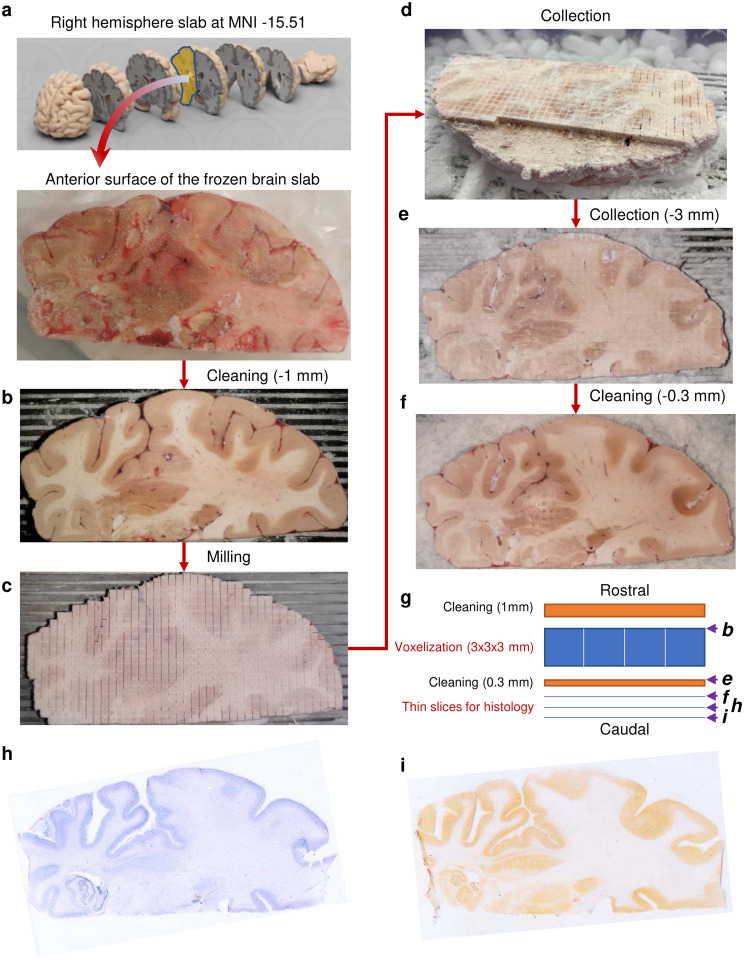
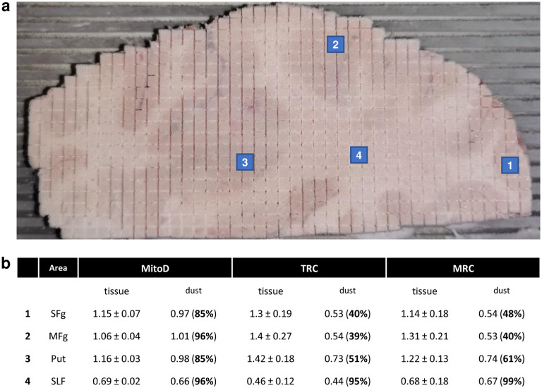
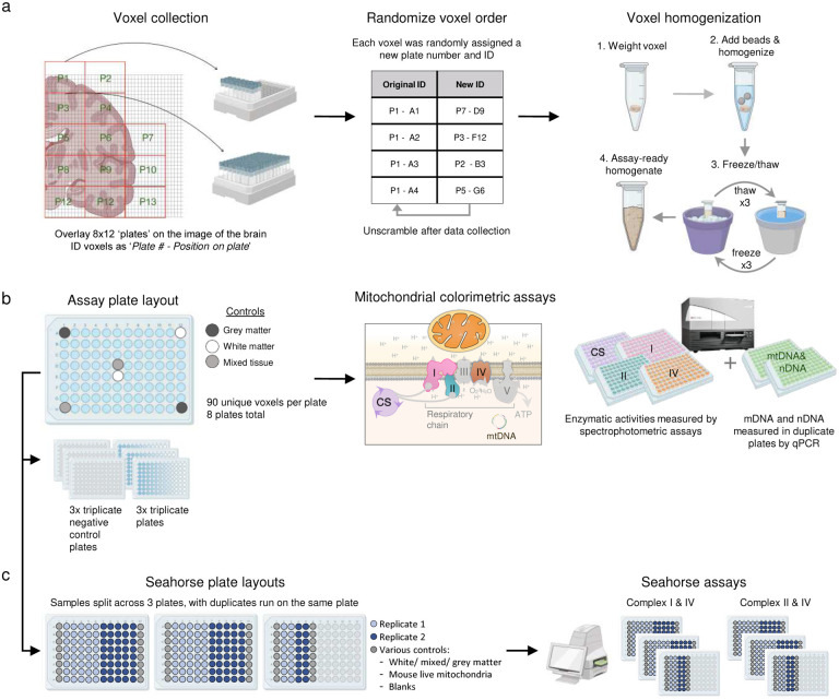
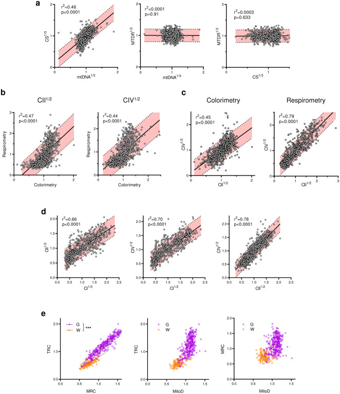
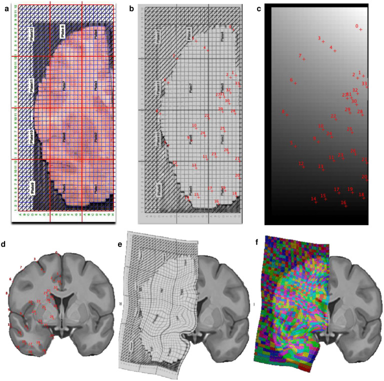
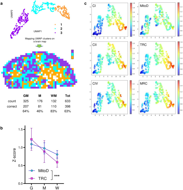
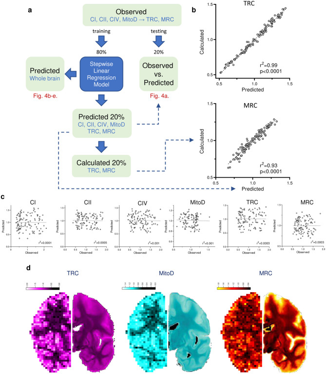
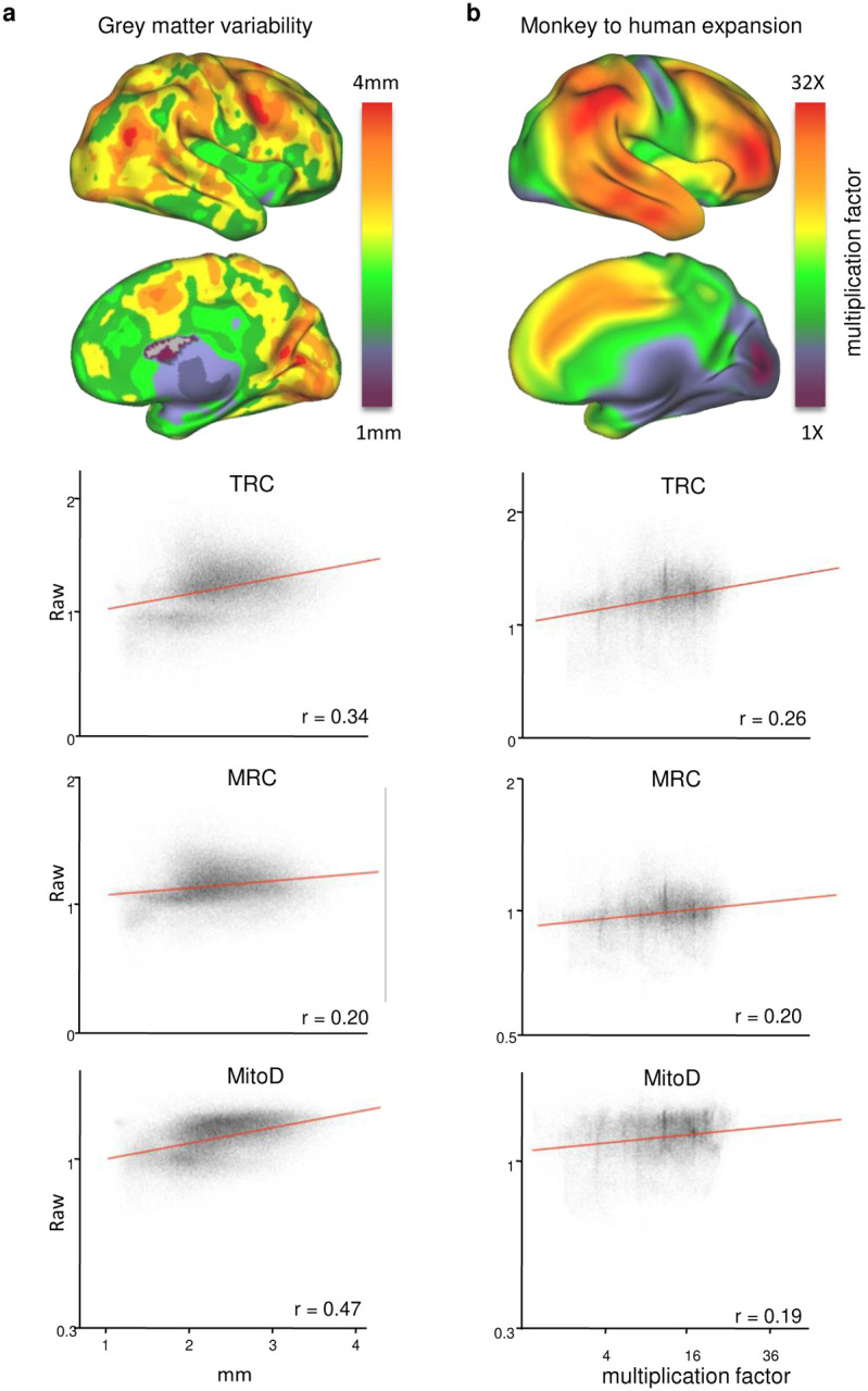
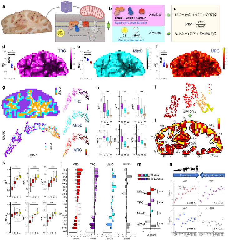
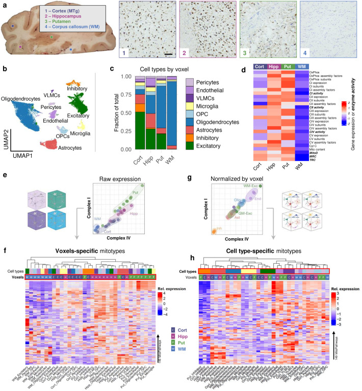
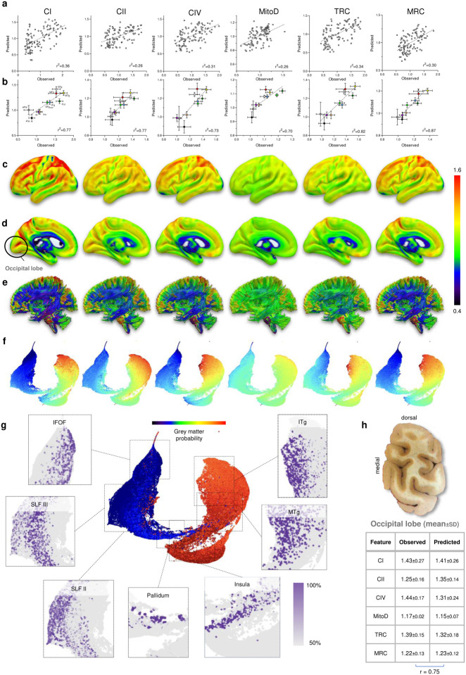
Mitochondrial oxidative phosphorylation (OxPhos) powers brain activity1,2, and mitochondrial defects are linked to neurodegenerative and neuropsychiatric disorders3,4, underscoring the need to define the brain's molecular energetic landscape5-10. To bridge the cognitive neuroscience and cell biology scale gap, we developed a physical voxelization approach to partition a frozen human coronal hemisphere section into 703 voxels comparable to neuroimaging resolution (3×3×3 mm). In each cortical and subcortical brain voxel, we profiled mitochondrial phenotypes including OxPhos enzyme activities, mitochondrial DNA and volume density, and mitochondria-specific respiratory capacity. We show that the human brain contains a diversity of mitochondrial phenotypes driven by both topology and cell types. Compared to white matter, grey matter contains >50% more mitochondria. We show that the more abundant grey matter mitochondria also are biochemically optimized for energy transformation, particularly among recently evolved cortical brain regions. Scaling these data to the whole brain, we created a backward linear regression model integrating several neuroimaging modalities11, thereby generating a brain-wide map of mitochondrial distribution and specialization that predicts mitochondrial characteristics in an independent brain region of the same donor brain. This new approach and the resulting MitoBrainMap of mitochondrial phenotypes provide a foundation for exploring the molecular energetic landscape that enables normal brain functions, relating it to neuroimaging data, and defining the subcellular basis for regionalized brain processes relevant to neuropsychiatric and neurodegenerative disorders.

Keywords: MRI; OxPhos; anatomical mapping; brain voxelization; mitochondria; neuroimaging; phenotyping; single-cell RNA sequencing.


Conflict of interest statement

Financial competing interests The authors have no competing interests to declare.

Figures

Extended Data Fig. 1 |
Extended Data Fig. 1 |. Workflow of tissue collection.
a, The right hemisphere coronal slab was mounted on a metal plate with an OCT compound with the top (anterior) surface of the slab parallel to the plate. b, After affixing the plate to the computer numerical control (CNC) cutting area, the top surface was cleaned with a 12.7 mm flat-tip drill bit rotating at 100 RPM and moving horizontally at 300 mm/sec. After cleaning 1 mm from the top, morphological brain structures were clearly visible and the surface was parallel to the plane of drill bit movement, ensuring that voxels will be of a uniform height. c, A 3×3 mm grid was milled with a 0.4 mm drill bit rotating at 10,000 RPM and moving horizontally at 250 mm/sec. During a single pass, 0.2 mm of the depth was milled, requiring 15 passes to reach the desired 3 mm of cut depth. Total milling time for a 130.8 × 61.25 mm hemisphere was ~5h. d, Fully milled slab was placed on dry ice. First, four samples of shavings were collected from the surface above one white and three gray areas (Extended Data Fig. 2). Next, shavings were gently removed from the surface with a brush and a pre-chilled scalpel and forceps were used to collect 703 individual voxels. e, Following sample collection, slab surface was cleaned once more with a 12.7 mm drill bit. f, The metal plate with the slab was then mounted on a freezing microtome and several 50 μm-thick cryosections were collected for histological evaluation. g, Summary of the steps during the collection of brain voxels and thin sections. Letters on the right refer to images shown on the corresponding panels. h and i, Thin brain section stained with Nissl to show neurons and glia either alone (h) or in combination with an immunostaining against neuronal nuclear antigen NeuN to highlight neuron-enriched areas (i).
Extended Data Fig. 2 |
Extended Data Fig. 2 |. Collection and analysis of tissue shavings.
a, Positions of collection sites of the four tissue shavings. Samples 1–3 were above the grey matter areas, while 4 was above a white matter area. b, Comparison of mitochondrial activities between the four ‘dust’ samples and corresponding tissue samples collected below after tissue voxelization. Values are mean ± SD. While all mitochondrial features (MitoD, TRC and MRC, see Fig 2c for definitions) were lower in all dust samples compared to tissue collected below, MitoD was less different between brain dust and tissue block. Moreover, in sample 4, brain dust and voxels features appear to be very similar, but this likely indicats that colorimetry and respirometry assays are at their detection limit when measuring mitochondria complex activities in the white matter.
Extended Data Fig. 3 |
Extended Data Fig. 3 |. Workflow for mitochondrial colorimetric and respiratory assays.
a, Brain voxel collection and preparation. b, Voxel plating and data collection for colorimetric mitochondrial assay and qPCR. c, Frozen tissue respirometry plate layouts derived from the assay plates in b to accommodate all samples and ran in duplicate. Samples were loaded into Seahorse plates at a constant volume rather than constant protein content.
Extended Data Fig. 4 |
Extended Data Fig. 4 |. Raw mitochondrial features measured by colorimetric and respirometry assays.
a, Image of the brain slab before voxelization. b, Distributions of non transformed values (i.e., values are in a linear scale) of citrate synthase (CS) activity, mitochondrial DNA (mtDNA) density and mitochondrial density (MitoD). c and d, Mapping of mitochondria complexes I, II and IV (CI, CII and CIV) activities measured by colorimetry (c) and respirometry (d) assays. e and f, Tissue Respiratory Capacity (TRC) and Mitochondria Respiratory Capacity (MRC) calculated from raw (non-transformed) values of enzymatic activities. Same maps derived from power transformed values of enzymatic activities are shown on Fig. 2e–f. Activity readouts were normalized to each group’s mean. Bar graphs on the left of the panel show distributions of repeated measures of control gray, white and mixed matter samples on different assay plates (i.e., data points are technical replicates of the same samples).
Extended Data Fig. 5 |
Extended Data Fig. 5 |. Volumetric transformation of mitochondrial parameters normalizes their distributions.
a, Distributions of complexes I, II and IV activities, CS activity and mtDNA density. Complex activities are averages from colorimetry and respirometry assays. b, Volumetric transformations of the data on a. Mitochondria density metrics and OxPhos complexes activities were calculated as averages of cube root and square root values from colorimetric and respirometry assays. c, Same data as b with voxels assigned to Gray matter (G, n=339) and White matter (W, n=169) clusters based on their anatomical location. Voxels with mixed identity (n=194) are not shown for simplicity.
Extended Data Fig. 6 |
Extended Data Fig. 6 |. Correlations between mitochondrial parameters assayed using different techniques.
a, CS activity and mtDNA density, which are related to mitochondria mass, are positively correlated. Because of the high variability in MitoTracker Deep Red (MTDR, a far-red fluorescent probe used to chemically mark and visualize mitochondria in cells) values, they correlated poorly with CS and mtDNA, thus MTDR was not used for the analysis. b and c, Relationship between CII and CIV activities measured by colorimetric and respirometry assays. d, Correlations between CI, CII and CIV activities (an average between colorimetric and respirometry assays). a-d, Pearson’s r2 values show how well datapoints follow the linear regression; p values indicate if the slope of the regression line is significantly different from zero; shaded areas represent 90% confidence interval. e, Relationship between TRC, MRC and MitoD values (see Fig. 2c for definitions) in gray and white matter voxels. *** - the slopes of linear regressions are different with p<0.001.
Extended Data Fig. 7 |
Extended Data Fig. 7 |. Mitochondrial features measured by colorimetry and respirometry assays.
a, Distributions of CS activity and mtDNA density. b, Measurements of mtDNA copy number (mtDNAcn) derived as a ratio of mitochondrial over nuclear DNA (mtDNA/nDNA). c and d. Mapping of CI, CII and CIV activities measured by colorimetry (c) and respirometry (d) assays. Because of the high variability of CI activities measured by colorimetry (c, top), these data were not used for TRC calculation. All values except mtDNAcn are normalized to each group’s mean. Bar graphs on the left of each panel show distributions of repeated measures of control Gray, White and Mixed matter samples on different assay plates (i.e., data points are technical replicates).
Extended Data Fig. 8 |
Extended Data Fig. 8 |. Morphing the partitioned brain slice into Montreal Neurological Institute (MNI) space.
a, Image of the partitioned brain slice with an overlaid milling grid. b, Conversion of the brain slice into Neuroimaging Informatics Technology Initiative (NIfTI) format and identification of 34 anatomical landmarks. c, Manual creation of NIfTI grid corresponding to the milling grid with the same coordinates. d, Identification of the anatomical landmarks as on b in the magnetic resonance imaging stereotaxic space (MNI152). e, Warping and deformation of the coordinates from b to d. f, Application of this deformation to c displayed in color onto the MNI152 for visual convenience. The following anatomical landmarks were identified: top of the interhemispheric fissure (0), surface (1) and deepest (2) point of the cingulate sulcus, surface (3) and deepest point (4) of the superior frontal sulcus (6), middle of the middle frontal gyrus (7), surface of the inferior frontal sulcus, middle surface of the inferior frontal gyrus (8), surface (5) and deepest point (9) of the lateral fissure, highest (10) and lowest (11) point of the circular insular sulcus, surface (12) and deepest point (13) of the superior temporal sulcus, surface (14) and deepest point (15) of the inferior temporal sulcus, surface (16) and deepest point (17) of the accessory temporopolar sulcus, surface (18) and deepest point (19) of the entorhinal sulcus, middle of the entorhinal cortex (20), most medial points of the amygdala (21), superior (22), inferior (23), lateral (24), and medial (25) putamen, most medial internal globus pallidus inferior (26), superior (27), inferior (28) lateral (29) and medial (30) caudate, highest point of the lateral ventricles (31), deepest point of the callosal sulcus (32) and middle of the cingulum gyrus (33).
Extended Data Fig. 9 |
Extended Data Fig. 9 |. Clustering of brain voxels by similarities of mitochondrial density and OxPhos activities.
a, Three visually defined UMAP clusters (upper) obtained after dimensionality reduction of mitochondrial features of all brain voxels (Fig. 2g) were used to predict whether voxels originated from GM, WM or a mixed sample (middle). The table lists prediction accuracy with the number of voxels of each type and the fractions that were identified correctly. Χ2(2, N=1031)=10.3, p<0.01. b, Both MitoD and TRC values were higher in GM than the WM voxels (same data as on Fig 2h are used; mean±SD), but the TRC decreases more than MitoD. ***- p<0.0001 by 2-way ANOVA (F1,1260=18.67). c, Distribution of z-score values of each mitochondrial feature on the UMAP plot of GM voxels only (Fig. 2i).
Extended Data Fig. 10 |
Extended Data Fig. 10 |. Histological evaluation of brain areas used for snRNAseq analysis.
Staining of 50 μm sections obtained after brain voxelization (see Extended Data Fig. 1) with Nissl stain (blue, neurons and glial cells) and NeuN (brown, neuronal cells). Two panels in black frames show Nissl-only stained sections with annotated cortical (layers I-II) and hippocampal (dentate gyrus, hilus and CA3) areas. The whole Nissl-stained brain section is shown on Extended Data Fig. 1h.
Extended Data Fig. 11 |
Extended Data Fig. 11 |. Workflow of data processing with stepwise linear regression model.
a, Voxels that had all 6 mitochondrial parameters (4 independent and 2 derived) and with a sum of GM and WM probabilities more than 70% (n = 539 ‘observed’ voxels) were randomly split into 80% learning (n = 431) and 20% testing (n = 108) datasets. A model was built by predicting each of the 6 mitochondrial values in the learning dataset using stepwise backward linear regression of neuroimaging values (Extended Data Table 1). The models were then applied to the testing dataset to verify predictions accuracy. Correlations between observed and predicted values of the testing dataset are shown on Fig. 4a. Next, the predictive models were extended to all the brain voxels of the MNI space to produce a whole brain estimated map for each of the mitochondrial values (Fig. 4b–e). b, Correlation between TRC and MRC values either predicted by the model or calculated from predicted CI, CII, CIV and MitoD values (see formulas on Fig. 2c). Strong correlation between predicted and calculated values for TRC and MRC shows the robustness of the model as it can accurately predict derived parameters (TRC and MRC) without knowledge of the independent readouts they were derived from (CI, CII, CIV and MitoD). c, Scatterplots of 20% out-of-sample prediction of mitochondrial profiles (same data as on Fig. 4a) after the pairing between voxels observed and predicted values was scrambled. Slopes of all linear regressions are not different from zero (p>0.7; Pearson’s r2 is shown on each graph). d, Predicted (right) vs. observed (left, same as Fig 2d–f) maps of TRC, MitoD and MRC values from the same coronal plane. Both sides show the right hemisphere (i.e., the predicted image is mirrored). Scale bars are in z-score units.
Extended Data Fig. 12 |
Extended Data Fig. 12 |. Higher mitochondrial activity in phylogenetically younger brain areas.
a-b, Comparison between predicted values and indirect measures of brain evolution such as grey matter variability (a) and monkey-to-humans areal expansion (b).
Fig. 1 |
Fig. 1 |. Overall strategy of brain voxelization and mapping.
a, Postmortem brain tissue was sectioned into ~2 cm thick coronal slabs, flash frozen in refrigerant HFC-134a and stored in −80°C freezer for 10 years (see Methods). b, A slab located at stereotactic Montreal Neurological Institute (MNI) coordinates 15.51 mm posterior to the center of the anterior commissure, was mounted on a computer numerical control (CNC) cutter operated in a −25C freezer room. c, The top surface was cleaned and leveled, and a square 3×3 mm grid was milled with a 0.4 mm drill bit to the depth of 3 mm. Brain voxels were manually collected, the surface cleaned once more, and several 50 μm cryosections were collected for histological evaluation. d, Each of the >700 samples was weighed, homogenized and ran through an array of biochemical tests, generating matrixes of mitochondrial features linked to voxel coordinates on the brain slice. e, Each voxel was characterized based on relative activities and abundance of mitochondrial complexes. f, Dimensionality reduction and clustering analysis was performed to identify different mitochondria phenotypes. Maps of mitochondrial features were registered onto a standard MNI space and correlated with average MRI readouts for the same brain regions. g, Finally, MRI data was used to predict mitochondrial features and to extend mitochondrial maps to the whole brain. h-j. Basic properties of collected voxels, including their (h) weight, (i) protein content and (j) nuclear DNA content. Histograms of each parameter values are shown on top and mapping of values on the brain slice at the bottom. Bar graphs on the left show repeated measurements of the corresponding values in control gray (G), white (W) and mixed (M) matter samples from the occipital lobe of the same brain that were used as normalization controls in the assay plates (see Extended Data Fig. 2).
Fig. 2 |
Fig. 2 |. Mitochondrial density and respiratory complexes activity assays.
a, Human brain slab before voxelization and schematic of the inner mitochondria membrane with respiratory chain (RC) complexes I-V. b, If organelle radii are normally distributed, activities of RC complexes that are proportional to the membrane surface should follow square root normal distribution. Citrate synthase (CS) and mtDNA levels are proportional to mitochondria volume and thus should follow a cube root normal distribution. c, Formulas for Tissue Respiratory Capacity (TRC), mitochondria density (MitoD) and Mitochondria Respiratory Capacity (MRC). Note that complex activities are normalized by tissue weight during sample preparation. d-f, Maps of TRC (d, derived from Extended Data Fig. 4c,d), MitoD (e, average of two panels on Extended Data Fig 4a), and MRC (f). Bar graphs on the left of each panel show distributions of repeated measures of control gray, white and mixed matter samples on different assay plates. g, Based on MNI space location (Extended Data Fig. 7), 633 voxels that had all 6 mitochondrial features (CI, CII, CIV, MitoD, TRC and MRC) were divided into gray (G, n=325), white (W, n=132) and mixed (M, n=176) matter clusters. Uniform Manifold Approximation and Projection (UMAP) algorithm was applied for dimension reduction. UMAP plots correlating clusters with physical location of each voxel (left) or z-score values of TRC, MitoD and MRC in each voxel (right). h, Bar (25 – 75 percentile) and whiskers (min and max) plots of mito features in voxels mapped to GM, WM and mixed tissue in MNI space. ***- all groups are significantly different from each other by one-way ANOVA with Tukey’s post-hoc test (p<0.001). i, UMAP plot and clusters of mitochondrial features of GM voxels. j, Mapping of voxel UMAP clusters on specific brain areas (see below for abbreviations). k, Comparison of mitochondrial features in four GM clusters identified on i. ***- significantly different from each other by one-way ANOVA with Tukey’s post-hoc test (p<0.001); for MitoD, only cluster 1 is different from all other clusters. l, Comparison of mitochondrial features in groups of voxels mapped into specific brain areas in the MNI space. Subcortical areas are shown in darker shades. m, Average z-scores of mitochondrial features in cortical and subcortical areas. ***- significantly different by t-test (p<0.01). n, Comparison between measured values and the known phylogenetically organization of main brain areas derived from comparative anatomy studies. Spearman’s rho is shown at the bottom-right. ePal, external pallidum; iPal, internal pallidum; BF, basal forebrain; C, caudate; Put, putamen. Areas also present in mammals with some close equivalent in reptiles: Piri, piriform cortex; H, hippocampus. Areas also present in mammals but not in reptiles: Ent, entorhinal cortex; Ins, insula; Cing, cingulate cortex. Neocortex in primates: ITg, inferior temporal gyrus; STg, superior temporal gyrus; SFg, superior frontal gyrus. Neocortex in humans: MTg, middle temporal gyrus; MFg, middle frontal gyrus.
Fig. 3 |
Fig. 3 |. snRNAseq analysis of selected voxels.
a, Location of voxels selected for snRNAseq analysis and their histological evaluation. Thin brain slices were stained with Nissl (blue, all nuclei) and immunolabeled for NeuN (brown, neuronal cells). Scale bar is 100 μm. b, UMAP plot of cell clusters identified by snRNAseq analysis of 4 voxels shows 9 major cell types. c, Cell type proportions in each of the 4 voxels. d, Heatmap of OxPhos pathway gene expression scores of each voxel (pseudobulk expression per sample), together with the activity measurements (bold). e, Correlations between complexes I and IV expression. Each data point represents pseudobulk expression of OxPhos subunits in each voxel/cell type and is color-coded by the voxel type. f, Heatmap of 149 mitochondrial pathways expression scores (see Supplementary File 1). Each column represents raw expression scores in a voxel/cell type color coded in the first two rows (same colors as in a for voxels and c for cell types). Note clustering of the samples by their voxel type. g, Correlations between complexes I and IV expression after z-score normalization of expression levels within each voxel type to account for region-specific differences. Each data point is color coded by its cell type. h, Heatmap of mitochondrial pathway expression scores in voxels/cell types after expression was normalized within each voxel. Clustering of samples by their cell type is now obvious.
Fig. 4 |
Fig. 4 |. Projected mitochondrial activities of the whole brain
a, Scatterplots of 20% out-of-sample prediction of mitochondrial profiles (see Extended Data Fig. 11). b, Correlations between observed and predicted mitochondrial features for brain areas rather than individual samples. Both ‘learning’ and ‘testing’ samples were used. n=5 voxels (ePal and iPal), 7 (MTg), 9 (MFg), 11 (IFgmed) 15 (H, Put and SFg), 27 (Ins), 33 (IFg). Slopes of all linear regressions on a and b are different from zero (p<0.0001; Pearson’s r2 is shown on each graph). c-e, Prediction of whole brain values for the lateral (c), medial (d) surfaces and the white matter connections (e, lateral view). 3D maps are available at https://identifiers.org/neurovault.collection:16418. f, UMAP embedding of the whole brain at 1 mm3 resolution, colors indicate mitochondrial activity profiles. g, UMAP plot of the whole brain with colors indicating the probability of each point being located in the white or gray matter. Insets show probabilities of voxels being in specific white matter (inferior frontooccipital fasciculus, superior longitudinal fasciculus) or gray matter (pallidum, insula, middle temporal gyrus, inferior temporal gyrus) brain structures (p < 0.0001 Bonferroni corrected for multiple comparisons). h, An image of the occipital lobe brain slab before milling (top) and summary table of mitochondrial features in the pooled gray matter OL samples used as loading controls (see Extended data Fig. 3). Predicted values were generated by averaging MRI-based model predicted mitochondrial metrics in 10 randomly selected GM voxels in the MNI space. Observed and predicted datasets are not different by 2-way ANOVA (F1,144=0.69, p=0.41); Pearson’s r is shown below the table.

Similar articles

References

    1. Shulman R. G., Hyder F. & Rothman D. L. Baseline brain energy supports the state of consciousness. Proc. Natl. Acad. Sci. U. S. A. 106, 11096–11101 (2009). - PMC - PubMed
    1. Zhang D. & Raichle M. E. Disease and the brain’s dark energy. Nat. Rev. Neurol. 6, 15–28 (2010). - PubMed
    1. Minhas P. S. et al. Restoring metabolism of myeloid cells reverses cognitive decline in ageing. Nature 590, 122–128 (2021). - PMC - PubMed
    1. Daniels T. E., Olsen E. M. & Tyrka A. R. Stress and Psychiatric Disorders: The Role of Mitochondria. Annu. Rev. Clin. Psychol. 16, 165–186 (2020). - PMC - PubMed
    1. Rosenberg A. M. et al. Brain mitochondrial diversity and network organization predict anxiety-like behavior in male mice. Nat. Commun. 14, 4726 (2023). - PMC - PubMed

Publication types

LinkOut - more resources