. 2024 Jan 25;15(2):1059-1073.
doi: 10.1364/BOE.511187. eCollection 2024 Feb 1.

Real-time line-field optical coherence tomography for cellular resolution imaging of biological tissue

Affiliations

Real-time line-field optical coherence tomography for cellular resolution imaging of biological tissue

Kai Neuhaus et al. Biomed Opt Express. .

Abstract

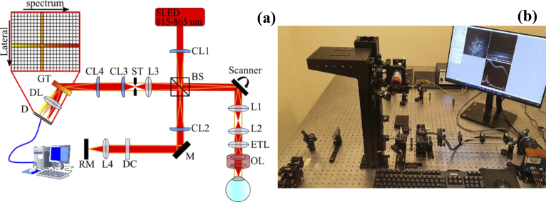
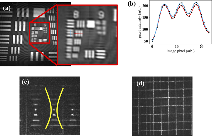
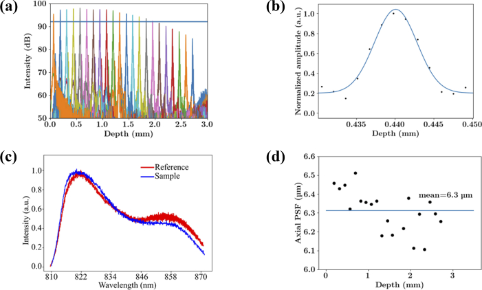
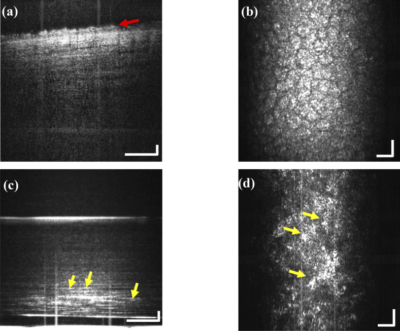
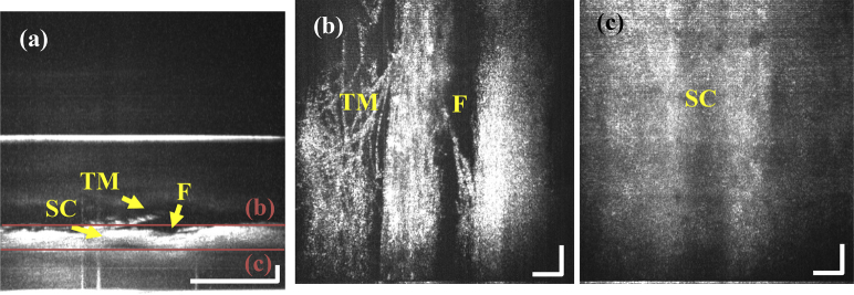
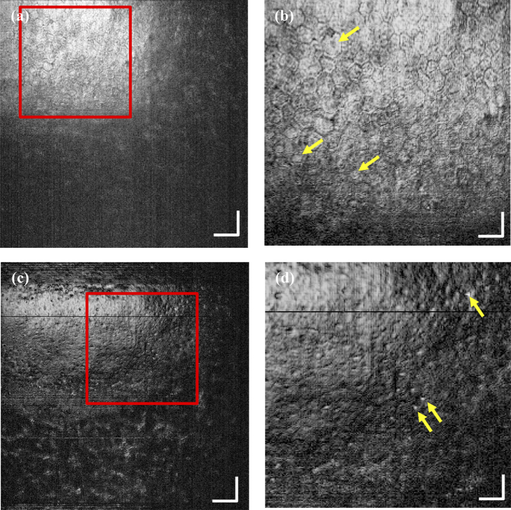
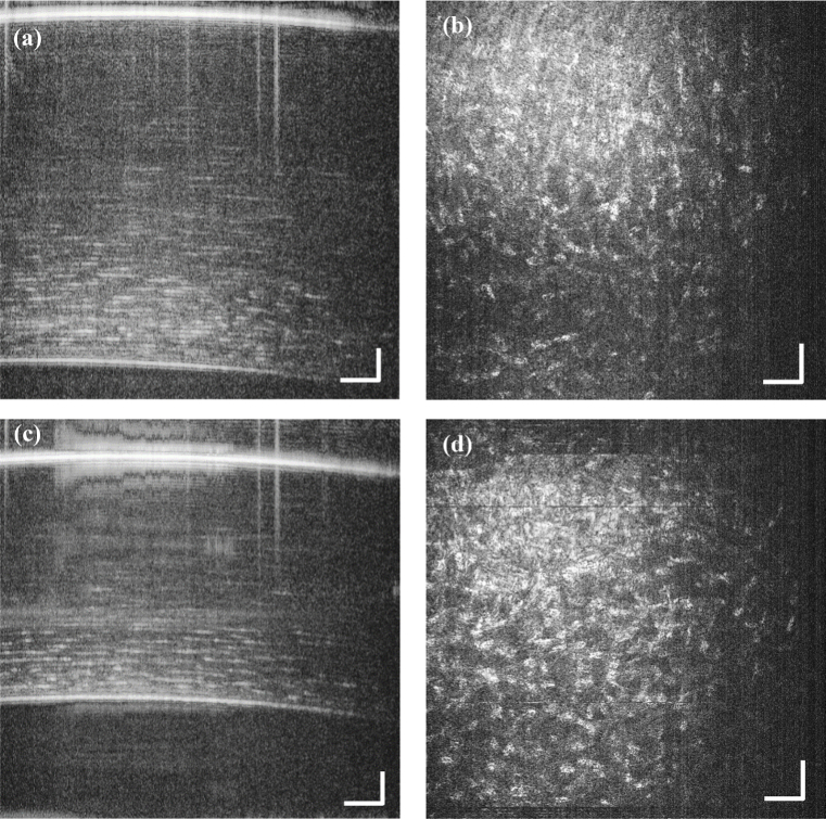
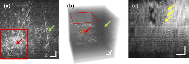
A real-time line-field optical coherence tomography (LF-OCT) system is demonstrated with image acquisition rates of up to 5000 B-frames or 2.5 million A-lines per second for 500 A-lines per B-frame. The system uses a high-speed low-cost camera to achieve continuous data transfer rates required for real-time imaging, allowing the evaluation of future applications in clinical or intraoperative environments. The light source is an 840 nm super-luminescent diode. Leveraging parallel computing with GPU and high speed CoaXPress data transfer interface, we were able to acquire, process, and display OCT data with low latency. The studied system uses anamorphic beam shaping in the detector arm, optimizing the field of view and sensitivity for imaging biological tissue at cellular resolution. The lateral and axial resolution measured in air were 1.7 µm and 6.3 µm, respectively. Experimental results demonstrate real-time inspection of the trabecular meshwork and Schlemm's canal on ex vivo corneoscleral wedges and real-time imaging of endothelial cells of human subjects in vivo.


Conflict of interest statement

David Huang: Optovue Inc. (F, I, P, R). These potential conflicts of interest have been reviewed and managed by OHSU. Other authors declare no relevant conflicts of interest related to this article.

Figures

Fig. 1.
Fig. 1.
(a) System schematics and (b) hardware setup of the real-time LF-OCT. In schematic (a) the beam is injected with a collimator generating a beam with 4 mm diameter from the SLED. The cylindrical lens (CL1) forms the lateral line illumination passing through the beam splitter (BS) with 50/50 splitting ratio, a second cylindrical lens (CL2), steering mirror (M), variable attenuation and dispersion compensation (DC), the reference lens (L4), and the reference mirror (RM). The sample arm is composed of the scanner, the beam expansion (L1, L2), a liquid lens (ETL), and the sample lens (OTL). The detector arm is comprised of a lens (L3), slit (ST), cylindrical lenses (CL3) and (CL4), the grating (GT), the detector lens (DL), and the detector (D). In (b) the SLED light source is visible in the background. The reference arm and mirror are visible at the lower left, and the spectrometer and high-speed camera at the lower right. The headrest is not shown. The 10X Mitutoyo lens is mounted at the upper right end of the vertical column.
Fig. 2.
Fig. 2.
(a) The lateral resolution was measured with a USAF target on element 2 of group 8. The fitted intensities for vertical and horizontal dimensions (markers indicate the pixel values) show that element 2 (b) can be discerned. A line width of 1.74 micrometer can well be identified. The images (c) and (d) were obtained with the 3D grid OCT phantom (Arden Photonics, APL-OP01) to evaluate the confocal gating (yellow) (c), and the lateral field of view (700 × 700) µm (d). The grid size of the phantom is (100 × 100) µm, and the vertical spacing between the gird layers is 75 µm.
Fig. 3.
Fig. 3.
(a) Fall-off characteristic of the unattenuated mirror signal for the axial PSF in air. The -6 dB fall-off (blue line) coincides at a depth of around 2 mm. The focus was positioned around 0.5 mm depth. (b) Gaussian fit for data points at a depth at about 440 µm, (c) the detected spectra for the reference and sample arm, and (d) all values for the FWHM at all measured depth positions, including the mean of 6.3 µm.
Fig. 4.
Fig. 4.
(a) B-frame of a human ex vivo corneoscleral sample showing the endothelial layer (red arrow). Note that the endothelial cells are abnormally swollen and appear enlarged. (b) En face projection at the same sample position shows the endothelial cells’ hexagonal pattern. (c) B-frame of the stroma of the same sample showing the thin and stretched keratocytes (yellow arrows), and (d) the en face projection. Note that larger patches may indicate clustering of keratocytes due to deformation of the cornea. The FOV for the B-frames (a) and (c) is about (150 × 500) µm (scale bars 30 µm) in width and height, and for the en face images (b) and (d) about (300 × 300) µm (scale bars 30 µm).
Fig. 5.
Fig. 5.
Tracking of the Schlemm’s canal. (a) B-frame FOV about (200 × 1000) µm (scale bars 60 µm) showing the layers (maroon colored) used for images (b) and (c). The layer (b) includes the trabecular meshwork (TM) and the layer (c) includes the Schlemm’s canal. Note that the fissure (F) in the upper layer (b) is slightly displaced relative to the Schlemm’s canal in layer (b). (b) En face image from showing the TM from the layer as indicated in (a). (c) En face image of the SC below the TM as indicated with layer (c) in subfigure (a). En face images (b) and (c) FOV is (300 × 300) µm (scale bars 30 µm).
Fig. 6.
Fig. 6.
In vivo real-time imaging snapshots of endothelial cells from two different human participants. The field of view for the left column of images (a) and (c) is (700 × 700) micrometers (scale bars 70 µm), and the right column (b) and (d) are the zoomed region (red) with a FOV of about (300 × 300) micrometers (scale bars 30 µm). Differences in contrast and cell size between the first participant, subfigure (a) and (b), compared to the second participant, subfigure (c) and (d), originate most likely from different depth positions of the focal plane and the limited DOF. The images for participant (c) and (d) are out of focus and bright spots of artifacts around the endothelial cells become visible (yellow arrows). Because due to the curvature of the cornea we can see how the keratocytes become increasingly visible at the bottom in image (c). Although for the current system configuration no image stabilization was attempted, the high imaging speed allows for multiple snapshots of full 3D image volumes allowing enhanced off-line inspection (see Visualization 1).
Fig. 7.
Fig. 7.
In vivo B-frames (a) and (c) from two different participants and corresponding en face images (b) and (d), about one hundred micrometers above the endothelial layer showing the distinct star shaped keratocytes. The width and height of the B-frames (a) and (c) is 700 and 800 micrometers respectively (scale bars 70 µm). The en face images have a field of view of 700 × 700 micrometers (scale bars 70 µm). We can appreciate the thicker (a) vs the thinner cornea (c). The focus for (a) and (c) was adjusted for the endothelial layer which causes increased intensity of the stratified stromal layers and keratocytes at the bottom of the images (a) and (c). Image (d) shows artefacts of horizontal image discontinuities due to occasional incomplete frame captures.
Fig. 8.
Fig. 8.
With the focus aligned below the epithelium and closer to the scleral edge we can increasingly identify larger nerve fibers (a) (see Visualization 4). The dimensions of (a) are 700 × 700 micrometers. With suitable post processing methods, we can allocate the nerve fiber structure in 3D, perform segmentation, and trace the path through the stroma (b). The colored arrows indicate the corresponding two strongly reflecting nerve fibers between the en face (a) and the 3D rendering (b). The dimensions of the cube (b) are 700 × 700 × 900 micrometers. Other structures were observed sporadically (yellow arrows) and are located in the center of the image (c). The field of view for (c) is about 450 × 450 micrometers after cropping. All scale bars are 70 µm.
Fig. 9.
Fig. 9.
Along the depth of the cornea different anatomical layers can be identified. In (a) the red boxes (b) and (c) are cutouts that are zoomed into in their corresponding figures (b) and (c). The yellow arrow in (a) indicates the highly reflecting tear film, then the corneal epithelium (EP), and the stroma (ST). Subfigure (b) shows a zoomed version with better visibility of the EP, the adjacent basal cell layer (BCL), the Bowman layer (BM), and stroma (ST). Some prominent highly reflecting elongated keratocytes (green arrows) are labeled in subfigure (b). Due to the focus at the epithelial layer the keratocytes towards the endothelial layer appear increasingly elongated. The Descemet’s membrane (DM) and the endothelial layer (EL) in (c) may be partially merged and potential side lobe artefacts of the OCT signal may obfuscate some of the layered structures. The FOV for (a) is vertically 900 and laterally 700 micrometers (scale bars 70 µm), and the zoomed regions (b) and (c) are approximately 220 micrometers vertically and 170 micrometers laterally (scale bars 25 µm).

Similar articles

Cited by

References

    1. Huang D., Swanson E. A., Lin C. P., et al. , “Optical coherence tomography,” Science 254(5035), 1178–1181 (1991).10.1126/science.1957169 - DOI - PMC - PubMed
    1. Tan B., Hosseinaee Z., Han L., et al. , “250 kHz, 1.5 µm resolution SD-OCT for in-vivo cellular imaging of the human cornea,” Biomed. Opt. Express 9(12), 6569–6583 (2018).10.1364/BOE.9.006569 - DOI - PMC - PubMed
    1. Hillmann D., Spahr H., Hain C., et al. , “Aberration-free volumetric high-speed imaging of in vivo retina,” Sci. Rep. 6(1), 35209 (2016).10.1038/srep35209 - DOI - PMC - PubMed
    1. Mazlin V., Xiao P., Scholler J., et al. , “Real-time non-contact cellular imaging and angiography of human cornea and limbus with common-path full-field/SD OCT,” Nat. Commun. 11(1), 1868 (2020).10.1038/s41467-020-15792-x - DOI - PMC - PubMed
    1. Lawman S., Zhang Z., Shen Y.-C., et al. , “Line Field Optical Coherence Tomography,” Photonics 9(12), 946 (2022).10.3390/photonics9120946 - DOI

LinkOut - more resources