. 2024 Feb 2;14(1):2780.
doi: 10.1038/s41598-024-53347-y.

On the nonlinearity of the foreperiod effect

Affiliations

On the nonlinearity of the foreperiod effect

Amirmahmoud Houshmand Chatroudi et al. Sci Rep. .

Abstract

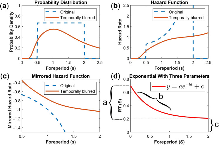
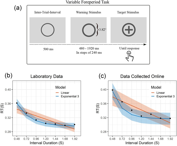
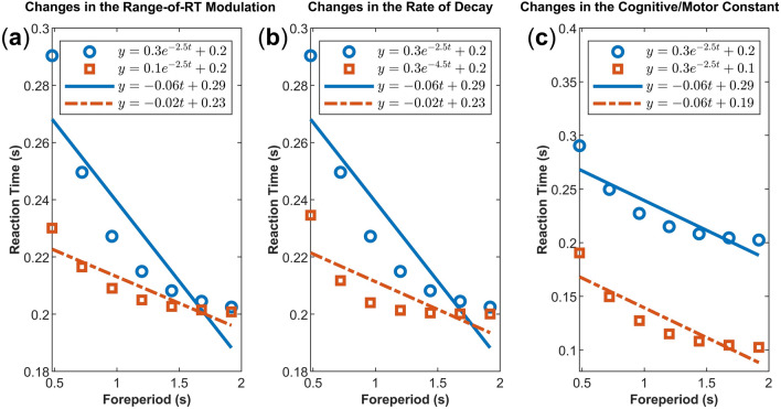
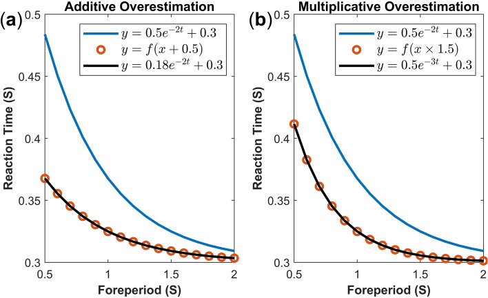
One of the frequently employed tasks within the implicit timing paradigm is the foreperiod task. The foreperiod is the time interval spanning from the presentation of a warning signal to the appearance of a target stimulus, during which reaction time trajectory follows time uncertainty. While the typical approach in analyzing foreperiod effects is based on linear approximations, the uncertainty in the estimation of time, expressed by the Weber fraction, implies a nonlinear trend. In the present study, we analyzed the variable foreperiod reaction times from a relatively large sample (n = 109). We found that the linear regression on reaction times and log-transformed reaction times poorly fitted the foreperiod data. However, a nonlinear regression based on an exponential decay function with three distinctive parameters provided the best fit. We discussed the inferential hazards of a simplistic linear approach and demonstrated how a nonlinear formulation can create new opportunities for studies in implicit timing research, which were previously impossible.


Conflict of interest statement

The authors declare no competing interests.

Figures

Figure 1
Figure 1
The blurring effect of applying Weber ratio to the objective hazard rate,. Panel (a) indicates a foreperiod range of 0.5 to 2 s, where the probability distribution of foreperiod intervals follows a uniform distribution. The blue dashed line represents the objective probability distribution. The red solid line shows the same distribution blurred according to the Weber ratio (φ = 0.49). Panel (b) shows the hazard function derived from panel (a). Note that the steep slope of blurred hazard rate in the beginning gradually decreases over longer durations. Panel (c) shows the inverted hazard function (mirrored; multiplied by − 1). The mirrored blurred hazard rate correlates positively with RT patterns in variable FP tasks. Note the steeper slope of mirrored blurred hazard rate in shorter durations. Panel (d) shows the potential nonlinear model for capturing the variable FP effect. Parameter ‘a’ in this exponential function is the y-intercept. This parameter corresponds to the amount participants can reduce their RT over the span of FP (the range of RT modulation). Parameter ‘b’ is the rate of decay, corresponding to the size of FP effect. Parameter ‘c’ is a constant (asymptote) corresponding to the motor/cognitive limitation. Thus, the assumption is that participants cannot improve their RT by reaching to zero, rather they will fixate at a constant RT due to motor/cognitive limitations. Note that the hazard function in panel (b) is derived from the continuous uniform probability density in panel (a). Therefore, the hazard function in panel (b) corresponds to the instantaneous rate of event occurrence given it has not occurred yet,. This value can exceed 1.
Figure 2
Figure 2
Task specifications (a) and group-level regression fits for data collected in the laboratory (b), and online (c). The shaded areas in (a,b) reflect 95% confidence bounds.
Figure 3
Figure 3
The interpretability problems of fitting a linear model to the variable FP effect. The blue circles are the RT points generated assuming an exponential function with three parameters. The lines are the best linear fits. In panel (a), the red squares show a change in the y-intercept of the exponential function (i.e. the range of RT modulation). The red dashed line represents the best linear fit. Compared to the best fit of the original data (the blue solid line), both the intercept and slope of the red dashed line have simultaneously changed. In panel (b), the red squares represent a change in the rate-of-decay of the original data (blue circles). Note that the slope and intercept of the linear fit (red dashed line) are both affected (compared to the blue solid line). In panel (c), the red squares indicate a change in the constant (asymptote) of the original exponential function. It is only in this scenario that the intercept of a linear function selectively captures the change without affecting the slope (generally representing a motor/cognitive cost, see text). Moreover, comparison of the red dashed lines between panel (a) and panel (b) illuminates that a linear model can remain insensitive to selective changes in the parameters of an underlying nonlinear function (in this case, y-intercept and rate-of-decay of an exponential function resulted in the same linear fits, i.e. red dashed lines with equal equations).
Figure 4
Figure 4
An exponential function with three parameters can selectively capture additive and multiplicative (under-) overestimation of time in a within-subject design. The blue line reflects an arbitrary reference function. The red circles represent RT under additive or multiplicative overestimations. The black line reflects the fit of the Exponential 3 function. Under the additive overestimation (panel (a)), foreperiod intervals are anticipated earlier than they should by a constant value (e.g. by 0.5 s as reflected by y=f(x+0.5); red circles relative to the blue reference line). Such an overestimation is selectively captured by changes in the y-intercept parameter (y-intercept parameter of the black line relative to the blue reference function). Under the multiplicative overestimation (panel (b)), foreperiod intervals are expected earlier than they should by a constant rate (e.g. by 50% as reflected by y=f(x×1.5); red circles relative to the blue reference line). Such an overestimation is independently captured by the rate-of-decay parameter of the Exponential 3 function (black line relative to the blue reference function).

Similar articles

Cited by

References

    1. Niemi P, Näätänen R. Foreperiod and simple reaction time. Psychol. Bull. 1981;89:133–162. doi: 10.1037/0033-2909.89.1.133. - DOI
    1. Woodrow H. The measurement of attention. Psychol. Monogr. 1914;17:i-158. doi: 10.1037/h0093087. - DOI
    1. Näätänen R. The diminishing time-uncertainty with the lapse of time after the warning signal in reaction-time experiments with varying fore-periods. Acta Psychol. (Amst.) 1970;34:399–419. doi: 10.1016/0001-6918(70)90035-1. - DOI - PubMed
    1. Näätänen R. Non-aging fore-periods and simple reaction time. Acta Psychol. (Amst.) 1971;35:316–327. doi: 10.1016/0001-6918(71)90040-0. - DOI
    1. Teichner WH. Recent studies of simple reaction time. Psychol. Bull. 1954;51:128–149. doi: 10.1037/h0060900. - DOI - PubMed