. 2023 Mar;20(200):20220700.
doi: 10.1098/rsif.2022.0700. Epub 2023 Mar 29.

Reinforced diffusions as models of memory-mediated animal movement

Affiliations

Reinforced diffusions as models of memory-mediated animal movement

William F Fagan et al. J R Soc Interface. 2023 Mar.

Abstract

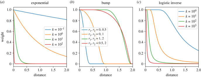
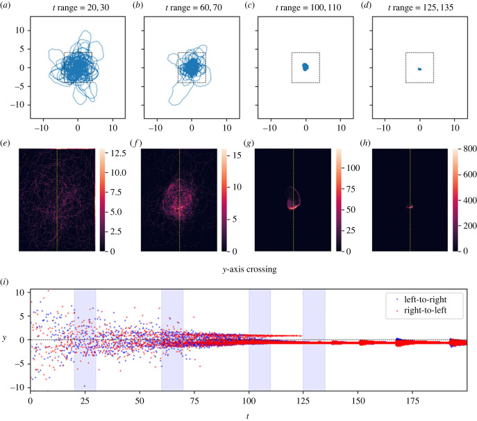
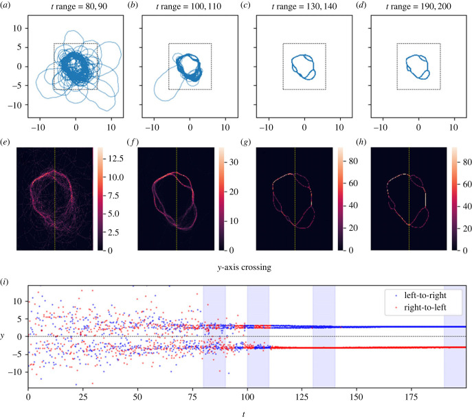
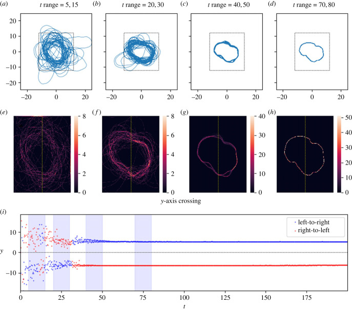
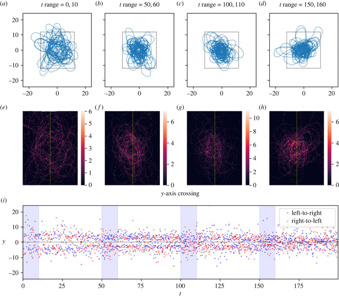
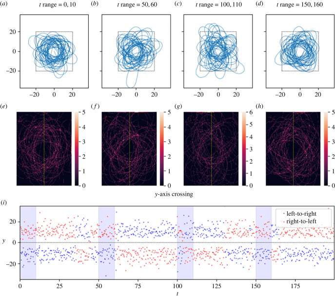
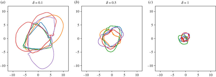
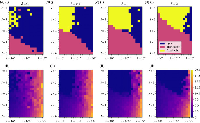
How memory shapes animals' movement paths is a topic of growing interest in ecology, with connections to planning for conservation and climate change. Empirical studies suggest that memory has both temporal and spatial components, and can include both attractive and aversive elements. Here, we introduce reinforced diffusions (the continuous time counterpart of reinforced random walks) as a modelling framework for understanding the role that memory plays in determining animal movements. This framework includes reinforcement via functions of time before present and of distance away from a current location. Focusing on the interplay between memory and central place attraction (a component of home ranging behaviour), we explore patterns of space usage that result from the reinforced diffusion. Our efforts identify three qualitatively different behaviours: bounded wandering behaviour that does not collapse spatially, collapse to a very small area, and, most intriguingly, convergence to a cycle. Subsequent applications show how reinforced diffusion can create movement trajectories emulating the learning of movement routes by homing pigeons and consolidation of ant travel paths. The mathematically explicit manner with which assumptions about the structure of memory can be stated and subsequently explored provides linkages to biological concepts like an animal's 'immediate surroundings' and memory decay.

Keywords: movement ecology; reinforced diffusion; reinforced random walk; spatial memory; time since last visit.


Conflict of interest statement

We declare we have no competing interests.

Figures

Figure 1.
Figure 1.
Candidate functions for the decay of memory. We interpret the distance over which the memory weight is approximately 1 as animals' ‘immediate surroundings' in which they have complete knowledge of the path traversed. Equations given in Methods.
Figure 2.
Figure 2.
In this figure, the track coalesces to a very tight distribution, which we call an ‘attractive point'. The track was allowed to evolve over 200 timesteps. Plots (ad) show the track in various timeframes. Plots (eh) are heatmaps showing the density of tracks by dividing a subset of x,y space (shown by black dashed lines in plots a–d) into cells and counting the number of tracks per cell. Each heatmap (eh) corresponds to the time window of the plot (a–d) above it. Plot (i) shows the times and y values of the crossings of the y-axis (marked by the dashed yellow line on the heatmaps), with direction indicated by colour. The four time windows of plots (a–h) are shown in light blue. Parameters as in table 2. After t ≈ 135, the distribution appears to expand and contract several times: this is the result of numerical instability of the solver in the vicinity of the highly attractive point (the system becomes ‘stiff'), a common issue with forward ODE solvers. Link to animation: https://youtu.be/bAJU2k6dVcU.
Figure 3.
Figure 3.
Here, the track coalesces into a cycle about the origin. Panels (ai) as in figure 2. At several points in space, the cycle separates from itself, then re-merges. However, these forking areas either shrink or disappear with time: between plots (c/d) and (g/h), the smallest fork (located at about 7 o'clock) disappears entirely, and the other three become shorter. Note that several times in plot (b), the track wanders off from the cycle for a time, then rejoins it. As can be seen in the plane-crossing plot (i), when the track rejoins the cycle, it sometimes starts moving along the cycle in the opposite direction. This implies that the long-term attraction of the path keeps the trajectory on the path, but does not dictate direction. Parameters as in table 2; the parameters here are the same as for figure 5, except that the long-term memory is 14% stronger in this case. This slight change produces this dramatically different behaviour. Link to animation: https://youtu.be/zIS2OJ-KjVw.
Figure 4.
Figure 4.
As in figure 3, here the trajectory forms a cycle about the origin, though in this case this happens much more quickly. While initially the cycle contains several forks, all of these disappear. Parameters as in table 2; note that the only difference in parameters between the cycle here and the distribution in figure 5 is the broadness of the distance function: a broader distance function (corresponding to greater ‘immediate surroundings') produces a clear reused path where a narrower one produces a distribution of tracks over space. Panels (a–i) as in figure 2. Link to animation: https://youtu.be/y3at1lwaE24.
Figure 5.
Figure 5.
Here, the effect of the long-term memory draws the trajectory into a tighter distribution than it exhibits initially, but this distribution persists going forward and does not collapse to an attractive point. Panels (a–i) as in figure 2. Link to animation: https://youtu.be/fi93coWPgmY.
Figure 6.
Figure 6.
Without long-term attraction to the past path, the trajectory again forms what we term a ‘distribution' (this is always the case when α = 0; figure 8). In this case, even without long-term attraction, the trajectory tends to orbit the origin: this is clear from the axis-crossing direction in plot (i). While this direction of rotation switches several times, the pattern of rotation is constant throughout. This rotation appears most clearly for ‘broad' distance functions (note in table 2 that k is lower for this figure than for figures 2–5). The function of long-term attraction, in these cases, is to take this existing rotational trend and condense it to a single reused closed path. Panels (a–i) as in figure 2. Parameters as in table 2.
Figure 7.
Figure 7.
Illustration of the diversity of possible cycles that can form under identical parameter conditions. In each plot, five trajectories are shown, each of which evolved under identical parameters, but with a unique random walk. Each plot has a different noise level (the parameter δ), whose impact on cycle size is clear. Parameters as in table 2.
Figure 8.
Figure 8.
Qualitative model output as a function of the relative intensities of the long- and short-term memories (I), the breadth of the distance function for memory (k) and the magnitude of white noise (δ). Each cell's information is derived from the results of a single trial under the given parameter conditions (315 parameter combinations in total). Row (i) shows the qualitative behaviours of the trajectories, corresponding to the movement track patterns illustrated in figures 2–6 and characterized in terms of the y-axis crossing values (plots i in figures 2–6). Row (ii) presents the standard deviation of the y-axis crossing values from the last 80 time units of each trial. Note that I > 1 corresponds to long-term attractive memory dominating whereas I < 1 corresponds to short-term aversive memory dominating. Note also that the k values decrease from left to right: this corresponds to an increase in the breadth of the distance function (i.e. an increase in the region a moving animal treats as its immediate surroundings; figure 1c). The colour bar and key are common to all panels in their respective rows. The dotted green square in (b(i)) indicates the 3 × 3 set of parameter conditions that was selected for additional trials to test whether different qualitative behaviours can form under the same parameter conditions (table 4 and figure 9 for results).
Figure 9.
Figure 9.
Each panel is a plane-crossing diagram of the same type as panel (i) in figures 2–6. Within the groups (a–c) and (d–f) all simulations use identical parameters (parameters as figure 8b, with I and k given here). However, in each of these groups, different trials with different random components produce qualitatively different results. Groups (a) and (b) form cycles (as indicated by the pair of groups of plane crossings), while (c) does not. Group (e) forms a cycle that collapses to a fixed point; (f) directly collapses to a fixed point without forming a cycle first; and (c) forms a cycle that remains stable. Table 4 shows the count of behaviour classifications (out of eight trials per parameter combination) for a region of the parameter space (indicated with a green square in figure 8b(i)) based on results like those shown here.

Similar articles

Cited by

References

    1. Fagan WF, et al. 2013. Spatial memory and animal movement. Ecol. Lett. 16, 1316-1329. (10.1111/ele.12165) - DOI - PubMed
    1. Mueller T, Fagan WF. 2008. Search and navigation in dynamic environments—from individual behaviors to population distributions. Oikos 117, 654-664. (10.1111/j.0030-1299.2008.16291.x) - DOI
    1. Bracis C, Mueller T. 2017. Memory, not just perception, plays an important role in terrestrial mammalian migration. Proc. R. Soc. B 284, 20170449. (10.1098/rspb.2017.0449) - DOI - PMC - PubMed
    1. Abrahms B, Hazen EL, Aikens EO. 2019. Memory and resource tracking drive blue whale migration. Proc. Natl Acad. Sci. USA 116, 5582-5587. (10.1073/pnas.1819031116) - DOI - PMC - PubMed
    1. Valeix M, Chamaillé-Jammes S, Loveridge AJ, Davidson Z, Hunt JE, Madzikanda H, Macdonald DW. 2011. Understanding patch departure rules for large carnivores: lion movements support a patch-disturbance hypothesis. Am. Nat. 178, 269-275. (10.1086/660824) - DOI - PubMed

Publication types

LinkOut - more resources