. 2023 Mar 17;18(3):e0277148.
doi: 10.1371/journal.pone.0277148. eCollection 2023.

Validation of a stereological method for estimating particle size and density from 2D projections with high accuracy

Affiliations

Validation of a stereological method for estimating particle size and density from 2D projections with high accuracy

Jason Seth Rothman et al. PLoS One. .

Abstract

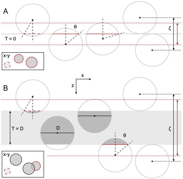
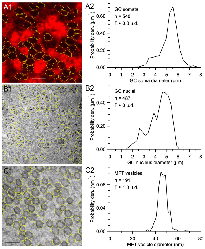
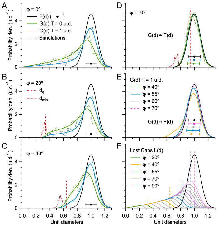
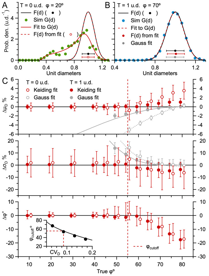
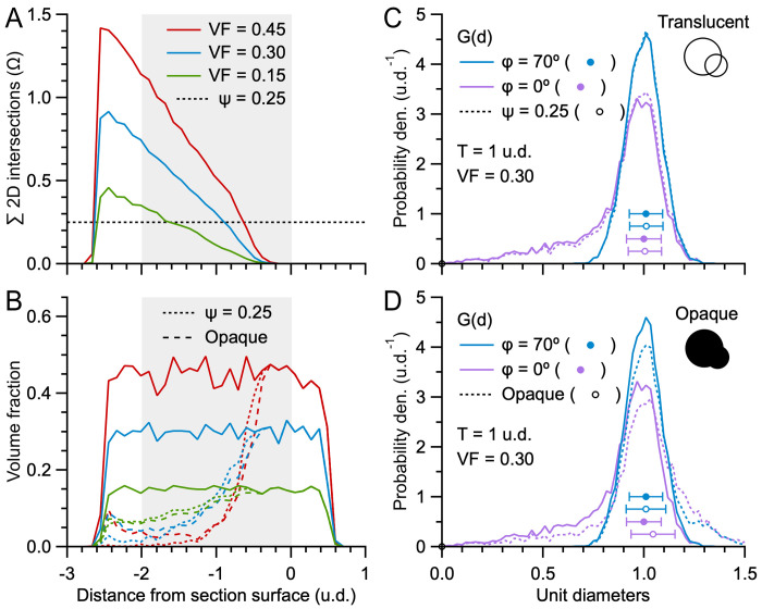
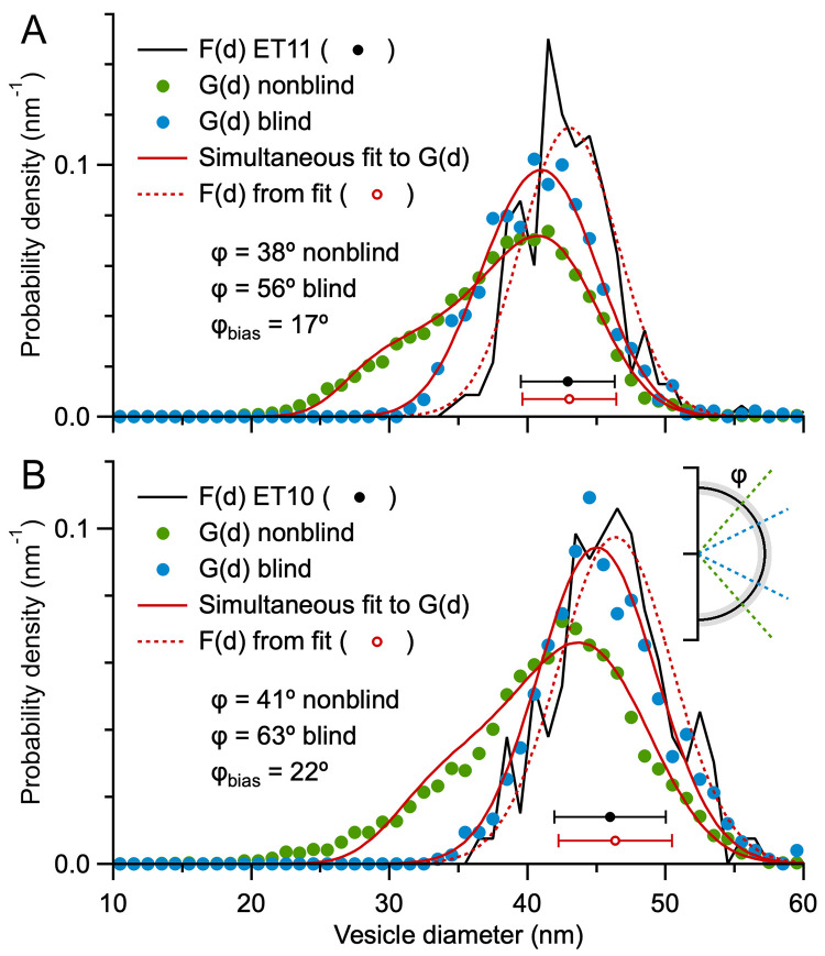
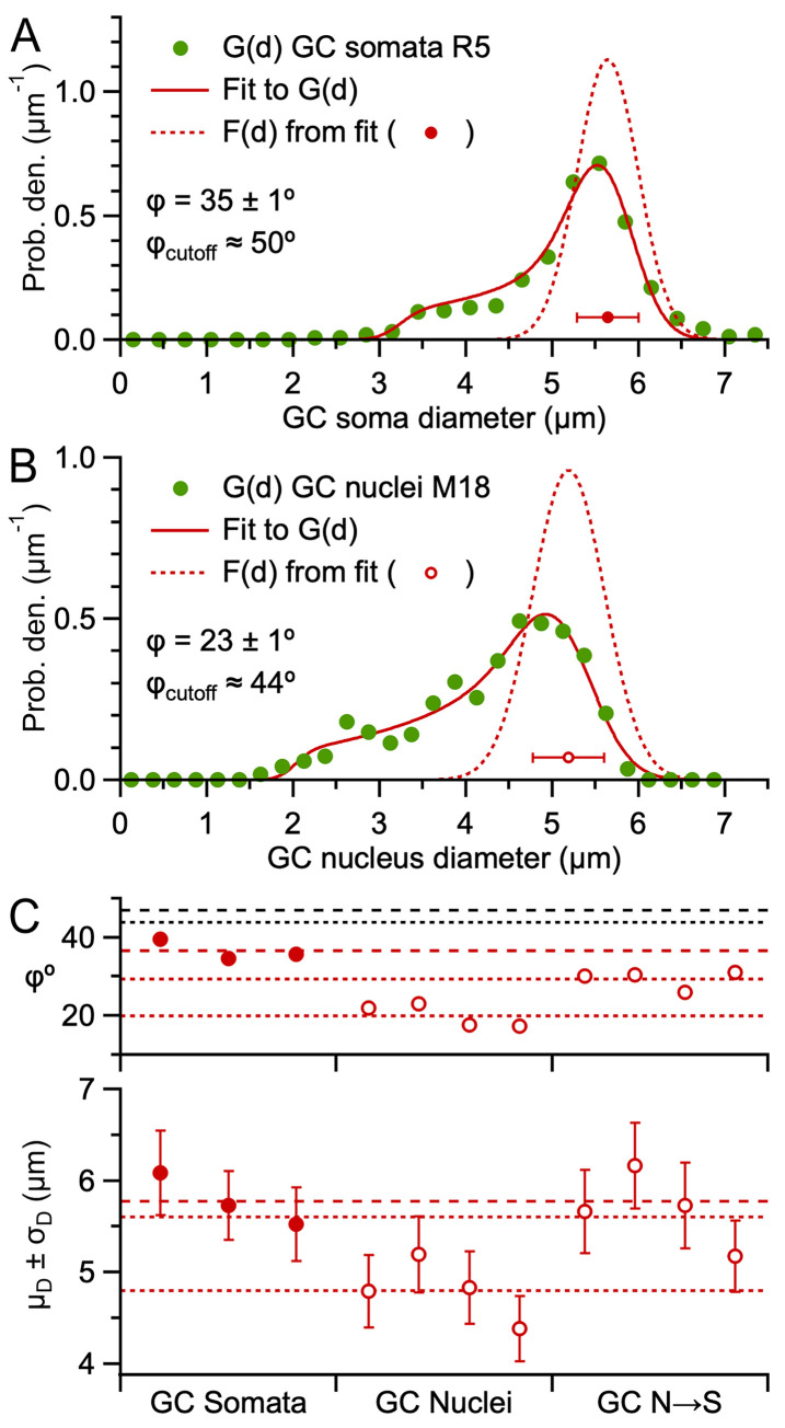
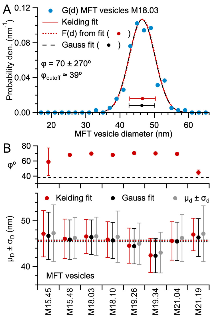
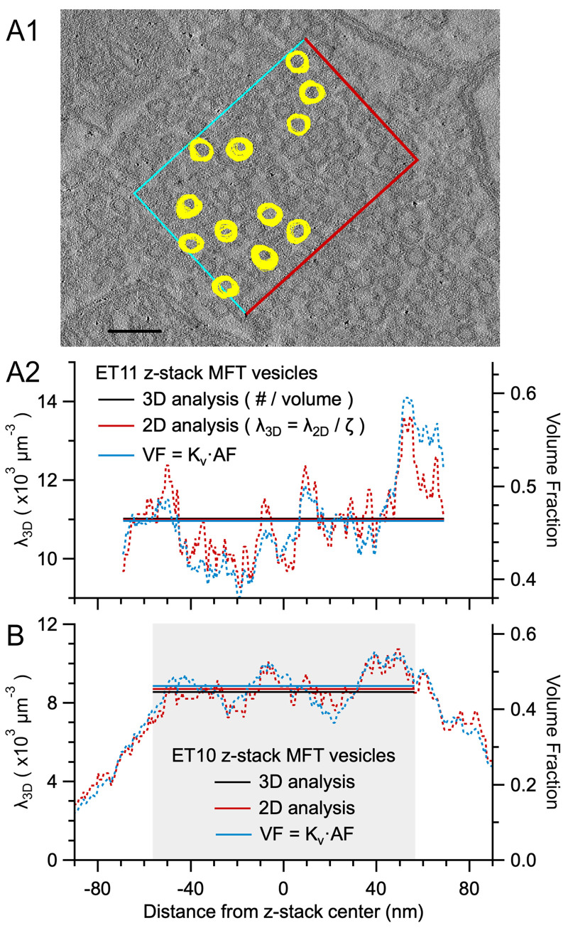
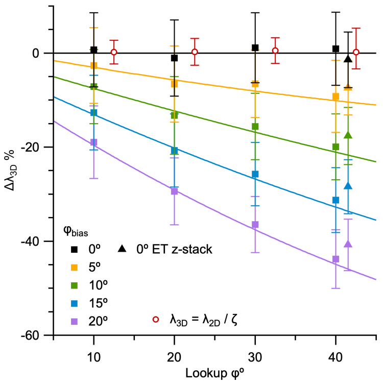
Stereological methods for estimating the 3D particle size and density from 2D projections are essential to many research fields. These methods are, however, prone to errors arising from undetected particle profiles due to sectioning and limited resolution, known as 'lost caps'. A potential solution developed by Keiding, Jensen, and Ranek in 1972, which we refer to as the Keiding model, accounts for lost caps by quantifying the smallest detectable profile in terms of its limiting 'cap angle' (ϕ), a size-independent measure of a particle's distance from the section surface. However, this simple solution has not been widely adopted nor tested. Rather, model-independent design-based stereological methods, which do not explicitly account for lost caps, have come to the fore. Here, we provide the first experimental validation of the Keiding model by comparing the size and density of particles estimated from 2D projections with direct measurement from 3D EM reconstructions of the same tissue. We applied the Keiding model to estimate the size and density of somata, nuclei and vesicles in the cerebellum of mice and rats, where high packing density can be problematic for design-based methods. Our analysis reveals a Gaussian distribution for ϕ rather than a single value. Nevertheless, curve fits of the Keiding model to the 2D diameter distribution accurately estimate the mean ϕ and 3D diameter distribution. While systematic testing using simulations revealed an upper limit to determining ϕ, our analysis shows that estimated ϕ can be used to determine the 3D particle density from the 2D density under a wide range of conditions, and this method is potentially more accurate than minimum-size-based lost-cap corrections and disector methods. Our results show the Keiding model provides an efficient means of accurately estimating the size and density of particles from 2D projections even under conditions of a high density.


Conflict of interest statement

The authors have declared that no competing interests exist.

Figures

Fig 1
Fig 1. Illustration of observed circular profiles when spherical particles are orthogonally viewed from above a planar or thick section.
A. Side view of a planar section (T = 0; gray line) transecting spherical particles (red solid lines). For simplicity, all particles have the same 3D diameter (D). Particles with their center above/below the section within a distance D/2 are observed as circular ‘caps’ in a horizontal projection (inset rectangle, top view, red circles) with apparent diameter d < D, where d = D·sinθ and θ is the cap angle (black dashed lines) that takes on values between 0°, where d = 0, and 90°, where d = D. Hence, those particles appearing within the projection have their center confined within a depth ζ = D (black double-headed arrow). However, due to experimental limitations, the smallest caps (with small θ) are not apparent, i.e. lost (red dashed lines). To account for lost caps, the Keiding model sets a minimum limit on θ (ϕ) such that caps are observed in the projection only if ϕ < θ < 90° [49]. In this case, ζ = D·cosϕ (red double-headed arrow; Eq 2). For planar sections, there are no projection overlaps (inset) and the total area fraction (AF) of the projections approximately equals the 3D volume fraction (VF) of the particles so long as there are relatively few lost caps. Because all particle centers fall above/below the planar section, all particles are considered caps. B. Same as A for a thick section (T = D). In this case, particles with their center within the section have a circular projection with d = D (black circles) and ζ = T + D·cosϕ. For thick sections and a high particle density, there are usually projection overlaps (inset) that make counting/outlining the projections more difficult; moreover, AF > VF, a condition known as overprojection.
Fig 2
Fig 2. Computing G(d) of GC somata and nuclei and MFT vesicles.
A1. Confocal image of a cerebellar section of a wild type (WT) rat (P30; from [6]). GC somatic plasma membranes were delineated via immunolabeling for Kv4.2. Outlines were drawn around those GC somata that were well delineated (yellow) and an equivalent diameter was computed from the area of each outline (darea). T ≈ 1.8 μm. Scale bar 10 μm. Image ID R5.SL2.1. A2. Probability density of 2D diameters (G(d)) computed from the GC soma diameters (0.30 μm bins) measured from the image in A1 plus 1 other image from the same z-stack. B1. Low-magnification TEM image of a cerebellar section of a WT mouse (P31). Outlines were drawn around the outer contour of visually identified GC nuclei (yellow). T ≈ 60 nm. Scale bar 10 μm. Image ID M18.N2.51. B2. G(d) computed from the GC nucleus diameters (0.25 μm bins) measured from the image in B1 plus 6 other images from the same mouse. C1. High-magnification TEM image of a MFT in the GC layer of the same mouse in B1. Outlines were drawn around the outer contour of the synaptic vesicles (yellow). T ≈ 60 nm. Because vesicles are semi-transparent, 2D overlaps do not necessarily preclude drawing their outline or counting. Scale bar 80 nm. Image ID M18.N2.03. C2. G(d) computed from the vesicle diameters (2 nm bins) measured from the TEM image in C1. For A1, B1 and C1 only a subregion of the outline analysis is shown.
Fig 3
Fig 3. Effect of section thickness and lost caps on G(d).
A. Probability density of 2D diameters (G(d)) computed via Eq 1, where ϕ = 0° and the probability density of 3D diameters (F(d)) is a Gaussian distribution with normalised mean (Eq 5; μD ± σD = 1.00 ± 0.09 u.d.; black line and circle ± error bars). For T = 0 u.d. (green line) conditions are that of Wicksell’s model [16] (Fig 1A) and for T = 1 u.d. (blue line) conditions are that of Bach’s model [38] (Fig 1B). Because no caps are lost, both G(d) have tails extending to d = 0 u.d. Dotted lines denote G(d) of equivalent Monte Carlo simulations computed from ~500 diameters using 0.04 u.d. bins. B–D. Same as A for ϕ = 20, 40 and 70°. Here, the tails of G(d) are limited to 0.3, 0.5 and 0.7 u.d. For ϕ = 70°, G(d) ≈ F(d) (green and blue circles denote μd ± σd) since most caps are lost. Comparison of the distribution of the minimum observed 2D diameter (dmin, red dotted line, computed from simulations for both T = 0 and 1 u.d., probability densities scaled by 0.07) to dϕ = μD·sinϕ (vertical red dashed line) shows dmin < dϕ, especially at larger ϕ. E. For ϕ > 55°, G(d) ≈ F(d). F. Distribution of lost caps, L(d), for ϕ = 5–90° in steps of 5° (gray and colored solid lines; Materials and Methods) compared to F(d) (black line). Vertical dashed lines denote dϕ. Note, L(d, ϕ = 90°) = G(d, ϕ = 0°).
Fig 4
Fig 4. The Keiding model accurately estimates F(d) and ϕ from G(d) for true ϕ < ϕcutoff (simulations).
A. Curve fit of Eq 1 (red solid line) to G(d) of the simulation in Fig 3B where T = 0 u.d. and ϕ = 20° (green circles; ~500 diameters). F(d) derived from the fit (red dashed line and circle) matches the true simulation F(d) (black line and circle) and fit ϕ matches true ϕ (ΔμD = -0.1%, ΔσD = +0.1%, Δϕ = +1°). B. Same as A for G(d) of the simulation in Fig 3D where T = 1 u.d. and ϕ = 70° (blue circles). Although there is a good match between estimated and true F(d), estimation errors ΔμD and ΔσD are larger than those in A and estimated ϕ < true ϕ (ΔμD = +0.9%, ΔσD = -4.4%, Δϕ = -9°). C. Average estimation errors ΔμD, ΔσD and Δϕ of Keiding-model fits to simulated G(d), as in A and B, for true ϕ = 10–80°, T = 0 and 1 u.d., CVD = 0.09 (red open and closed circles; μΔ ± σΔ for 100 repetitions per ϕ). Red dashed lines denote ϕcutoff (~55°; Eq 8) above which G(d) ≈ F(d) and true ϕ becomes indeterminable. For comparison, results are shown for Gaussian fits to the same G(d) (Eq 5; gray circles) and 2D statistics μd ± σd (gray lines). Data shifted ±0.8° to avoid overlap. Asymmetrical error bars indicate skewed distributions (Materials and Methods). Inset: ϕcutoff vs. CVD for simulations (black circles) and Eq 8 (black line; n = 500 diameters). See S1–S5 Figs in S1 File.
Fig 5
Fig 5. Effects of projection overlaps for thick sections.
A. Sum of 2D projection overlaps (Ω) as a function of distance from the surface of a simulated section for particle VF = 0.15, 0.30 and 0.45 (green, blue and red lines) where Ω > 1 indicates a particle’s projection is likely to be completely overlapping with projections of other particles closer to the section surface. Histograms were computed using particle z-center points and 0.1 u.d. bins. Gray background denotes section thickness (T = 2 u.d.). The distributions extend 0.5 u.d. below the section because of caps (Fig 1B). Black dotted line denotes upper limit ψ = 0.25 for B and C. For simplicity, ϕ = 0°. B. VF of those particles appearing in a simulated projection as a function of distance from the surface of each section (T = 2 u.d.) for transparent particles (solid lines; control, ψ = ∞), semi-transparent particles (dotted lines; a particle is removed from the projection if its Ω > 0.25) and opaque particles (dashed lines; bottom-dwelling particles are merged with top-dwelling particles if -1 < α < 0; Materials and Methods). VF = 0.15, 0.30 and 0.45 as in A. The effect of semi-transparent and opaque particles is to reduce the effective T. Histograms were computed using particle z-center points and 0.1 u.d. bins; counts were converted to VF using the equivalent bin volume (geometry Areaxy multiplied by bin z-width) and particle diameter distribution. For simplicity, ϕ = 0°. C. Comparison of simulated probability density of 2D diameters (G(d); 0.02 u.d. bins) for transparent and semi-transparent particles (ψ = ∞ and 0.25; solid vs. dotted lines) shows little difference for two extreme conditions of lost caps (ϕ = 0° and 70°; purple and blue). In these simulations, projection overlaps did not affect estimates of their size (inset). Circles and error bars denote Keiding-model fit parameters μD ± σD. T = 1 and VF = 0.30. D. Comparison of simulated G(d) for transparent and opaque particles (solid vs. dotted lines). For opaque particles, overlapping projections with -1 < α < 0 were treated as a single projection with larger area (inset), thereby creating a positive skew in G(d). For AD, average histograms were computed from 20 sections, ~500 particles per section.
Fig 6
Fig 6. The Keiding model accurately estimates F(d) and ϕ from G(d) for true ϕ < ϕcutoff (vesicles ET11).
A. One of 261 serial images of a 3D ET reconstruction (ET11) of a cerebellar MFT section 138 nm thick. 271 vesicles, including 101 caps, were tracked and outlined through multiple z-planes and their darea computed as a function of z-plane number (z#). This image shows outlines for 8 representative vesicles, overlaid with outlines from images above and below. Scale bar 50 nm. B. Vesicle xy-radius (½darea) vs. z-depth (colored lines) with vesicle centers (z0) aligned at z = 0; caps are not displayed. Black semi-circle and shading denote μD ± σD = 42.9 ± 3.4 nm for all measured 3D diameters (D; n = 233). Black dotted lines and shading denote measured ϕ: μϕ ± σϕ = 41.5 ± 7.2° (n = 403, measures of north and south poles, including caps). Parameters z0 and D were estimated via a curve fit to Eq 10 and ϕ = sin-1min/D), where δmin is the minimum darea at a given pole (S6A Fig in S1 File). Average fit E = 1.00 ± 0.16 (n = 233) where estimated Sz = 0.53 nm (S6B Fig in S1 File). Fits to the smallest caps were not included (n = 38). C1. Minimum 2D diameter of a given vesicle (δmin) vs. D (circles; n = 403) with line fit (black line; χ2 = 5957, r = 0.4, R2 = 0.1) and Keiding-model fit (red solid line; δmin = D·sinϕ; fit ϕ = 41.0 ± 0.3°; χ2 = 6105, r = 0.4, R2 = 0.3). The smallest δmin (dmin = 19 nm; red dashed line) is a poor match to the data. C2. Same as C1 but for ϕ = sin-1min/D) with line fit (black line; r = -0.1, R2 = 0.02) and μϕ = 41.5° (red solid line). C3. Probability density (per °) of measured ϕ in C2 (black circles; probability per degree) with Gaussian fit (gray line; Eq 5) and fit ϕ (red line) and ϕcutoff from D (black dashed line; ~63°; Eq 8). Note, the difference between the fit and measured ϕ (Δϕ = -3°) can partially be accounted for by an estimated +1° discretization error of measured ϕ (S6D Fig in S1 File) and a -0.3° error of fit ϕ from assuming a fixed ϕ (S10C Fig in S1 File). D. Measured F(d) (black line and circle; 1 nm bins; see B) vs. G(d) (green circles; n = 13,914 outlines; 1 nm bins). A curve fit of Eq 1 to G(d) (red solid line; μD = 42.9 ± 0.1 nm, σD = 3.4 ± 0.1 nm, ϕ = 38.4 ± 0.3°; T fixed to 0 nm) resulted in estimated F(d) (red dotted line and circle) nearly the same as measured F(d) and estimated ϕ nearly the same as μϕ (C3). See S6–S10 Figs in S1 File.
Fig 7
Fig 7. Comparison of G(d) computed blind versus nonblind reveals a large bias in particle cap detection for MFT vesicles (ϕbias ≈ 20°).
A. Probability density of 2D diameters (G(d)) computed via a nonblind vesicle detection (green circles; ET11; Fig 6D) versus a blind vesicle detection (blue circles). Both G(d) were simultaneously curve fitted to Eq 1, where parameters μD and σD were shared, revealing a 17° bias in ϕ (red solid lines; μD = 43.0 ± 0.1 nm, σD = 3.5 ± 0.1 nm, nonblind ϕ = 38.3 ± 0.5°, blind ϕ = 55.5 ± 0.7°). As in Fig 6D, estimated F(d) (red dotted line and circle) is similar to measured F(d) (black solid line and circle). For the blind analysis, there were 889 diameters measured from 18 z-planes (z# = 1–260) spaced 5–15 nm apart, analysed in random order. B. Same as A for ET10 (S8D Fig in S1 File). The simultaneous curve fit revealed a 22° bias in ϕ (red solid lines; μD = 46.4 ± 0.1 nm, σD = 4.1 ± 0.1 nm, nonblind ϕ = 40.9 ± 0.7°, blind ϕ = 63.3 ± 1.3°). For the blind analysis, there were 751 diameters measured from 30 z-planes (z# = 51–236) spaced 2–7 nm apart, analysed in random order. Inset cartoon depicts the bias in ϕ along the axial axis of a vesicle.
Fig 8
Fig 8. Estimates of F(d) and ϕ from G(d) of cerebellar GC somata and nuclei.
A. Curve fit of Eq 1 (red solid line) to the G(d) of rat GC somata in Fig 2A2 (green circles) resulting in estimates for F(d) (red dotted line and circle), ϕ and ϕcutoff (Eq 9). B. Same as A for the G(d) of mouse GC nuclei in Fig 2B2. C. Parameters μD ± σD (bottom) and ϕ (top) from Keiding-model fits to G(d) of GC somata for 3 rats (red closed circles; S12 Fig in S1 File; weighted averages with respect to number of tissue sections), G(d) of GC nuclei for 4 mice (red open circles; S13 Fig in S1 File; pooled diameters from 6–7 TEM images per mouse) and the same G(d) of GC nuclei scaled to somata dimensions (N→S). Red dashed and dotted lines denote averages across the 3 rats and 4 mice, respectively. Black dashed and dotted lines denote average estimated ϕcutoff for somata and nuclei (~47 and 44°).
Fig 9
Fig 9. Estimates of F(d) and ϕ from G(d) of MFT vesicles.
A. Curve fit of Eq 1 (red solid line) to the G(d) of mouse MFT vesicles in Fig 2C2 (blue circles) resulting in estimates for F(d) (red dotted line and circle), ϕ and ϕcutoff (Eq 9). A Gaussian fit to the same G(d) (black dashed line) overlaps the Keiding-model fit and μD ± σD of both fits overlap (red and black circles) indicating G(d) ≈ F(d). B. Parameters μD ± σD (bottom) and ϕ (top) from Keiding-model curve fits to G(d) of MFT vesicles for 4 mice, 2 MFTs per mouse (red circles; S15 Fig in S1 File), compared to μD ± σD from Gaussian fits (black circles) and μd ± σd computed from 2D diameters. Overlapping distributions again indicate G(d) ≈ F(d). Dotted lines (bottom) denote averages. Black dashed line (top) denotes average estimated ϕcutoff (~38°); all estimated ϕ are considered inaccurate. Error bars of ϕ denote fit errors, 6 of which are not shown since they are off scale. See S16 Fig in S1 File.
Fig 10
Fig 10. The Keiding model accurately estimates λ3D from λ2D for true ϕ < estimated ϕcutoff (simulations).
A. Average error in section z-depth over which particle center points are sampled (Δζ) vs. true ϕ (top) for simulations in Fig 4C for T = 0 and 1 u.d. (red open and closed circles) where estimated ζ was computed via Eq 2 using true μD, ϕ and T and ‘true’ ζ = λ2D3D using measured λ2D and true λ3D. B. Average error in 3D particle density (Δλ3D) vs. true ϕ (middle) for the same simulations, computed via estimated and true λ3D, where estimated λ3D was computed via Eq 3 (λ3D = λ2D/ζ) using measured λ2D and estimated μD and ϕ from Keiding-model fits to the simulated G(d). Red dashed line denotes estimated ϕcutoff (~43°; Eq 9). One error bar at true ϕ = 55° is off scale (+56%). C. Average error in volume fraction (ΔVF) vs. true ϕ (bottom) for the same simulations, computed via estimated and true VF, where estimated VF = Kv·AF (Eq 14). For A, B and C, results are also shown for transparent particles (black solid line; ψ = 0.25) and opaque particles (black dashed line) in thick sections (T = 1 u.d.; Fig 5), showing estimated ζ was larger than true ζ when projection overlaps hindered particle counting, creating a large underestimation of λ3D and VF. However, for opaque particles, the bias was larger for λ3D than VF since an overlap in two projections reduced the particle count by one, but only partially reduced the AF (overlapping projections coalesce into one). Data x-scales were shifted ±0.8° to avoid overlap. See S18 Fig in S1 File.
Fig 11
Fig 11. The Keiding model accurately estimates λ3D from λ2D for true ϕ < estimated ϕcutoff (vesicles).
A1. One of 261 serial ET images (ET11) of a cerebellar tissue section. A ROI (0.45 × 0.32 μm; Areaxy = 0.144 μm2) was placed within a large cluster of MFT vesicles and those vesicles that obeyed the inclusive/exclusive borders (blue/red; n = 271) were tracked and outlined through multiple z-planes. Because the analysis includes vesicle caps on the top/bottom of the reconstruction, the vesicle sampling space of the volume of interest (VOI) extends above/below the section such that ζ = 170 nm (Fig 1B; Eq 2; 3D measures: T = 138 nm, μD = 42.9 nm, μϕ = 42°) giving VOI = 0.025 μm3. Here, outlines for 12 representative vesicles are overlaid with outlines from images above and below. Scale bar 100 nm. A2. Vesicle λ3D (left axis) and VF (right axis) computed within the ROI in A1. For the 3D analysis, λ3D = N3D/VOI = 11,022 μm-3 (black solid line). For the first 2D analysis, λ3D = λ2D/ζ (Eq 3) computed for each z-plane (red dotted line) and the sum of all z-planes (red solid line), where λ2D is the number of outlines per ROI area and ζ = 34 nm computed via Keiding-model estimates μD and ϕ (Fig 6D). For the second 2D analysis, VF = Kv·AF (Eq 14) computed for each z-plane (blue dotted line) and the sum of all z-planes (blue solid line; 0.46), where Kv = 1.07 and AF is the sum of all vesicle outline areas per ROI area. Both the measured ϕ (42°) and estimated ϕ (38°) are less than estimated ϕcutoff (51°; Eq 9). Left and right axes are equivalent scales for μD ± σD = 42.9 ± 3.4 nm, the measured F(d). B. Same as A2 for ET10. Gray shading denotes the axial subregion where the 3D analysis and averages were computed (Materials and Methods). Left and right axes are equivalent scales for μD ± σD = 46.0 ± 4.0 nm. See S19 Fig in S1 File.
Fig 12
Fig 12. Estimation errors of the 3D density computed via the disector method for different degrees of bias due to blind-versus-nonblind cap detection.
Average Δλ3D computed from Monte Carlo simulations of the disector method, where a particle-detection bias was simulated by increasing ϕ of the reference section (a blind cap detection) with respect to the lookup section (a nonblind cap detection) for ϕbias = 0–20° (colored squares; ϕref = ϕlookup + ϕbias; ~500 particles per reference section). Thickness of the reference and lookup sections was 0.3 u.d. An equivalent disector analysis using the ET11 z-stack data gave similar results (triangles; lookup ϕ = 42°). Average Δλ3D for the simulations in Fig 10B are shown for comparison (red open circles; T = 0 u.d.; λ3D = λ2D/ζ; x-scale is true ϕ and is shifted 2.5° to avoid overlap) highlighting the higher levels of accuracy compared to the disector method, i.e. smaller confidence intervals (σΔ).
Fig 13
Fig 13. Methods workflow for estimating the 3D size and density of spherical particles from their 2D projection.
Workflow diagram describing the sequence of steps for estimating F(d) (μD ± σD) and ϕ from G(d), and λ3D from λ2D, where G(d) and λ2D are computed from a 2D projection of randomly distributed particles in a section of thickness T. Two check marks indicate a negligible bias and small confidence interval compared to one check mark. Final estimates of λ3D can be converted to VF using estimated μD ± σD (Eq 4) and compared to that computed via the relation VF = Kv·AF (Eq 14). Estimated ϕ is compared to estimated ϕcutoff, computed via fit parameters μD and σD (Eq 9). Green and red arrows denote ‘yes’ and ‘no’ of conditional statements.

Similar articles

References

    1. Elias H, Hennig A, Schwartz DE. Stereology: applications to biomedical research. Physiol Rev. 1971. Jan;51(1): 158–200. doi: 10.1152/physrev.1971.51.1.158 - DOI - PubMed
    1. Royet JP. Stereology: a method for analyzing images. Prog Neurobiol. 1991;37(5): 433–74. doi: 10.1016/0301-0082(91)90009-p - DOI - PubMed
    1. Borges-Merjane C, Kim O, Jonas P. Functional electron microscopy, ‘“Flash and Freeze,”‘ of identified cortical synapses in acute brain slices. Neuron. 2020. Dec 9;108(5): 1011. doi: 10.1016/j.neuron.2020.11.015 - DOI - PMC - PubMed
    1. Murthy VN, Sejnowski TJ, Stevens CF. Heterogeneous release properties of visualized individual hippocampal synapses. Neuron. 1997. Apr;18(4): 599–612. doi: 10.1016/S0896-6273(00)80301-3 - DOI - PubMed
    1. Rothman JS, Kocsis L, Herzog E, Nusser Z, Silver RA. Physical determinants of vesicle mobility and supply at a central synapse. eLife. 2016. Aug 19;5: e15133. doi: 10.7554/eLife.15133 - DOI - PMC - PubMed

Publication types