

In vivo magnetic resonance P-Spectral Analysis With Neural Networks: 31P-SPAWNN
- PMID: 36161342
- PMCID: PMC9828468
- DOI: 10.1002/mrm.29446
In vivo magnetic resonance P-Spectral Analysis With Neural Networks: 31P-SPAWNN
Abstract
Purpose: We have introduced an artificial intelligence framework, 31P-SPAWNN, in order to fully analyze phosphorus-31 ( P) magnetic resonance spectra. The flexibility and speed of the technique rival traditional least-square fitting methods, with the performance of the two approaches, are compared in this work.
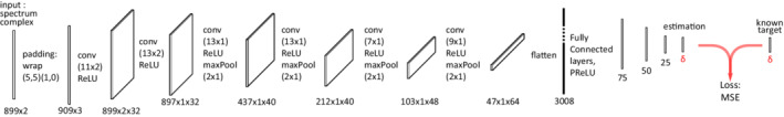
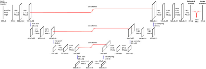
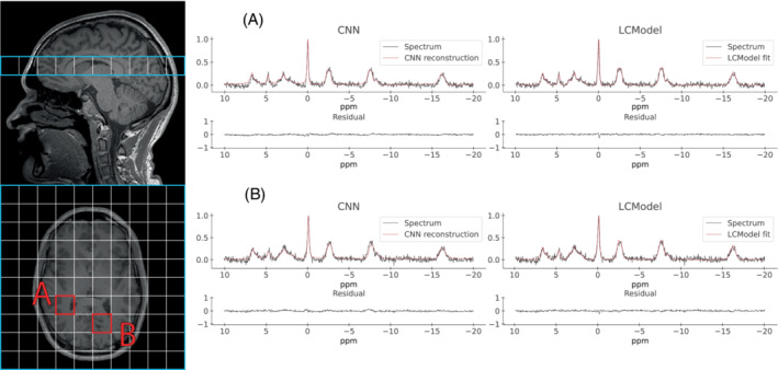
Theory and methods: Convolutional neural network architectures have been proposed for the analysis and quantification of P-spectroscopy. The generation of training and test data using a fully parameterized model is presented herein. In vivo unlocalized free induction decay and three-dimensional P-magnetic resonance spectroscopy imaging data were acquired from healthy volunteers before being quantified using either 31P-SPAWNN or traditional least-square fitting techniques.
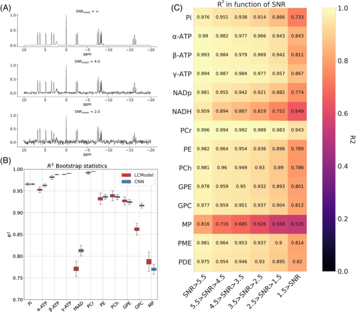
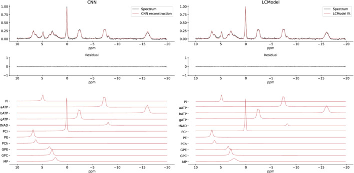
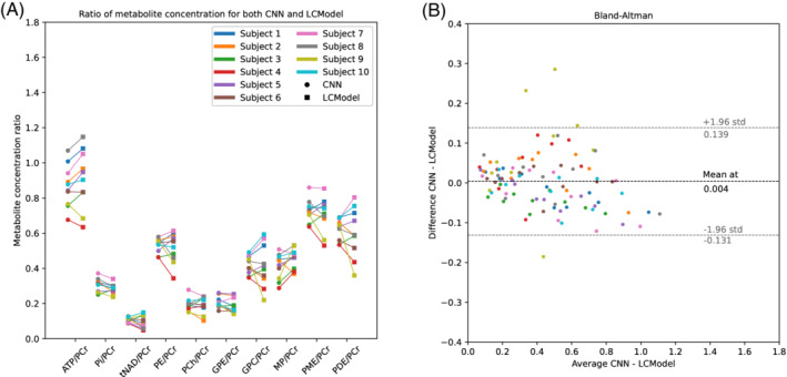
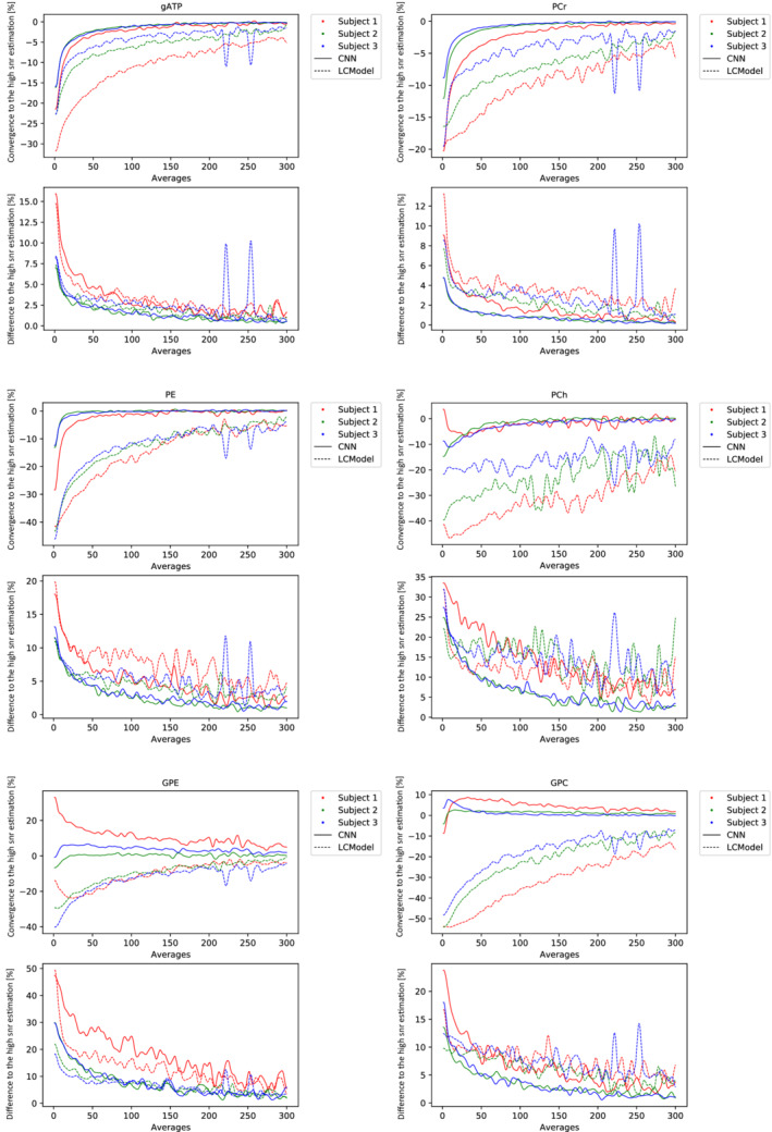
Results: The presented experiment has demonstrated both the reliability and accuracy of 31P-SPAWNN for estimating metabolite concentrations and spectral parameters. Simulated test data showed improved quantification using 31P-SPAWNN compared with LCModel. In vivo data analysis revealed higher accuracy at low signal-to-noise ratio using 31P-SPAWNN, yet with equivalent precision. Processing time using 31P-SPAWNN can be further shortened up to two orders of magnitude.
Conclusion: The accuracy, reliability, and computational speed of the method open new perspectives for integrating these applications in a clinical setting.
Keywords: LCModel; convolutional neural network; deep learning; in vivo; phosphorus magnetic resonance spectroscopy.
© 2022 The Authors. Magnetic Resonance in Medicine published by Wiley Periodicals LLC on behalf of International Society for Magnetic Resonance in Medicine.
Figures

Similar articles
-
Comparison of convolutional-neural-networks-based method and LCModel on the quantification of in vivo magnetic resonance spectroscopy.MAGMA. 2024 Jul;37(3):477-489. doi: 10.1007/s10334-023-01120-z. Epub 2023 Sep 15. MAGMA. 2024. PMID: 37713007
-
Intact metabolite spectrum mining by deep learning in proton magnetic resonance spectroscopy of the brain.Magn Reson Med. 2019 Jul;82(1):33-48. doi: 10.1002/mrm.27727. Epub 2019 Mar 12. Magn Reson Med. 2019. PMID: 30860291
-
Assessment of quantitative artificial neural network analysis in a metabolically dynamic ex vivo 31P NMR pig liver study.Magn Reson Med. 1997 Nov;38(5):840-4. doi: 10.1002/mrm.1910380522. Magn Reson Med. 1997. PMID: 9358460
-
Absolute quantification of phosphorus metabolite concentrations in human muscle in vivo by 31P MRS: a quantitative review.NMR Biomed. 2007 Oct;20(6):555-65. doi: 10.1002/nbm.1192. NMR Biomed. 2007. PMID: 17628042 Review.
-
Methodological standardization for a multi-institutional in vivo trial of localized 31P MR spectroscopy in human cancer research. In vitro and normal volunteer studies.NMR Biomed. 2004 Oct;17(6):382-91. doi: 10.1002/nbm.915. NMR Biomed. 2004. PMID: 15386624 Review.
Cited by
-
Sodium Hydrosulfide Treatment During Porcine Kidney Ex Vivo Perfusion and Transplantation.Transplant Direct. 2023 Oct 30;9(11):e1508. doi: 10.1097/TXD.0000000000001508. eCollection 2023 Nov. Transplant Direct. 2023. PMID: 37915463 Free PMC article.
-
Reproducible Research Practices in Magnetic Resonance Neuroimaging: A Review Informed by Advanced Language Models.Magn Reson Med Sci. 2024 Jul 1;23(3):252-267. doi: 10.2463/mrms.rev.2023-0174. Epub 2024 Jun 19. Magn Reson Med Sci. 2024. PMID: 38897936 Free PMC article. Review.
References
-
- Reto B, Dieter M, Ernst M, Peter B. Assessment of absolute metabolite concentrations in human tissue by 31P MRS in vivo part II: muscle, liver, kidney. Magn Reson Med. 1994;32:453‐458. - PubMed
-
- Chmelik M, Schmid A, Gruber S, et al. Three‐dimensional high‐resolution magnetic resonance spectroscopic imaging for absolute quantification of 31P metabolites in human liver. Magn Reson Med. 2008;60:796‐802. - PubMed
-
- Webb Graham A, ed. Methods and applications of phosphorus NMR spectroscopy in vivo. Annual Reports on NMR Spectroscopy. Vol 75. Academic Press; 2012.
-
- Rudin M, ed. In‐Vivo Magnetic Resonance Spectroscopy III: In‐Vivo MR Spectroscopy: Potential and Limitations. Springer Berlin Heidelberg; 1992.
Publication types
MeSH terms
Substances
LinkOut - more resources
Full Text Sources
