. 2022 Aug 3:16:931121.
doi: 10.3389/fncom.2022.931121. eCollection 2022.

Nonlinear optimal control of a mean-field model of neural population dynamics

Affiliations

Nonlinear optimal control of a mean-field model of neural population dynamics

Lena Salfenmoser et al. Front Comput Neurosci. .

Abstract

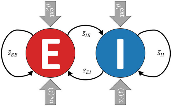
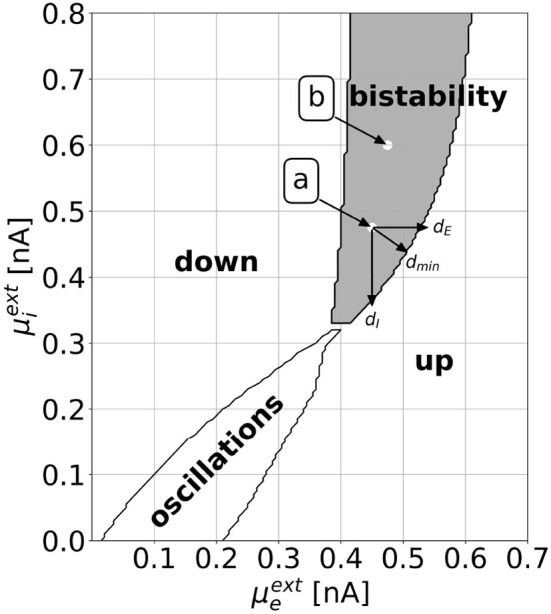
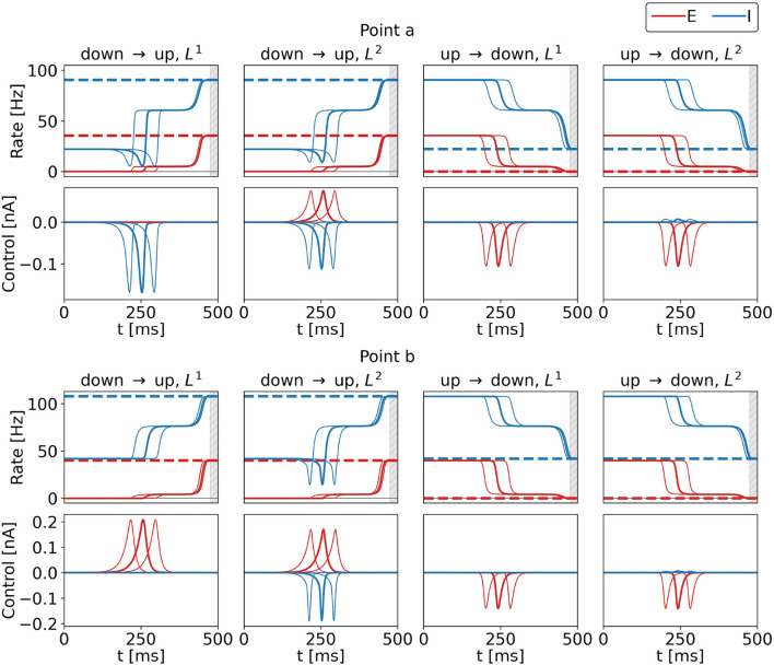
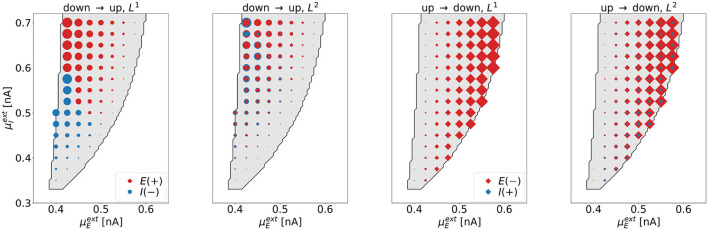
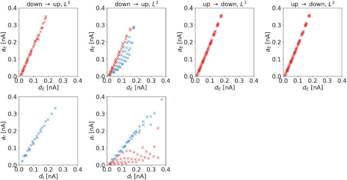
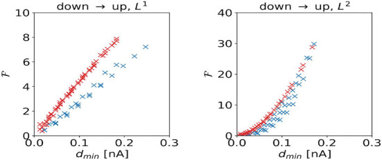
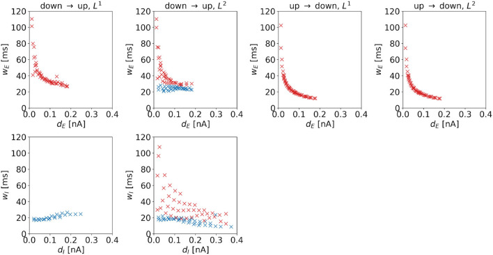
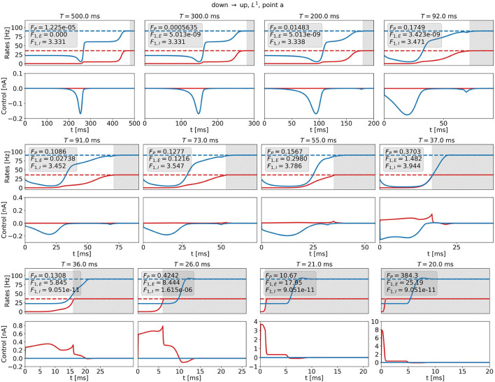
We apply the framework of nonlinear optimal control to a biophysically realistic neural mass model, which consists of two mutually coupled populations of deterministic excitatory and inhibitory neurons. External control signals are realized by time-dependent inputs to both populations. Optimality is defined by two alternative cost functions that trade the deviation of the controlled variable from its target value against the "strength" of the control, which is quantified by the integrated 1- and 2-norms of the control signal. We focus on a bistable region in state space where one low- ("down state") and one high-activity ("up state") stable fixed points coexist. With methods of nonlinear optimal control, we search for the most cost-efficient control function to switch between both activity states. For a broad range of parameters, we find that cost-efficient control strategies consist of a pulse of finite duration to push the state variables only minimally into the basin of attraction of the target state. This strategy only breaks down once we impose time constraints that force the system to switch on a time scale comparable to the duration of the control pulse. Penalizing control strength via the integrated 1-norm (2-norm) yields control inputs targeting one or both populations. However, whether control inputs to the excitatory or the inhibitory population dominate, depends on the location in state space relative to the bifurcation lines. Our study highlights the applicability of nonlinear optimal control to understand neuronal processing under constraints better.

Keywords: bistability; control of neural dynamics; delay differential-algebraic equations (DDAEs); neural mass models; nonlinear optimal control; nonlinear population dynamics.


Conflict of interest statement

The authors declare that the research was conducted in the absence of any commercial or financial relationships that could be construed as a potential conflict of interest.

Figures

Figure 1
Figure 1
A simplified visualization of the model. The excitatory and the inhibitory subpopulations are recurrently coupled and receive external background inputs μE,Iext and time-varying external control currents uE,I(t).
Figure 2
Figure 2
The dynamical landscape of the mean-field EI EIF model. Depending on the mean background inputs μEext and μIext, we observe a down state, an up state, an oscillatory regime, or a bistable regime, where down and up states coexist. We choose two locations, which we call point a (μEext=0.45nA,μIext=0.475nA) and point b (μEext=0.475nA,μIext=0.6nA), for which we show explicit results in Section 3. We define the horizontal, vertical, and shortest distance to the regime boundary as dE, dI, and dmin, respectively. This definition can be applied both for the distances to the up regime, as shown in the figure, and to the down regime.
Figure 3
Figure 3
Flowchart summarizing the gradient descent procedure for computing the optimal control u*(t). After initializing the algorithm with an initial guess for the control u0(t), six steps are performed within each iteration. The algorithm terminates if the change of control between subsequent iterations is below a predefined threshold value ϵu in all components and for all points of time.
Figure 4
Figure 4
Control inputs and population rates for three different initializations for the four control tasks and for points a (top row) and b (bottom row) marked in the state space diagram of Figure 2. Bold lines show results obtained for the standard initialization, and the lines to the right (left) show results with the initialization pulse shifted by 40 ms (−40 ms). The top rows show the firing rates of the excitatory (red) and inhibitory (blue) population as a function of time, bottom rows show the corresponding optimal control currents, uE in red, uI in blue. From left to right, the columns show the results for the DU1-, DU2-, UD1-, and UD2-task. The respective target rates are indicated by the dashed lines. The simulation duration is T = 500 ms. During the last 20 ms, precision is penalized (gray shaded area). The numerical values for the costs are FDU1 = 3.3312, FDU2 = 3.5516, FUD1 = 2.1462, and FUD2 = 2.2901 at point a, and FDU1 = 5.0064, FDU2 = 10.9004, FUD1 = 2.6569, and FUD2 = 3.5209 at point b for all three initializations.
Figure 5
Figure 5
Dynamical variables as a function of time for the DU1-task, when optimal control is applied. Parameters correspond to point a shown in Figure 2. Variables related to the excitatory (inhibitory) population are plotted in red (blue). We show the optimal control input to the inhibitory population in each plot as the thin, dashed, blue line (uE = 0). All dynamical variables reach a plateau state between t≈ 250 ms and t ≈ 400 ms.
Figure 6
Figure 6
The dimensionality of the optimal control signals at selected points (μEext,μIext) in the bistable regime. The four panels correspond to the four control tasks. Each marker represents one point in state space, for which the optimal control was computed. We indicate the excitatory (inhibitory) control amplitude with red (blue) markers. The area of the markers scales with the respective amplitude of the optimal control signal. For the down-to-up tasks (first and second panel), red circles correspond to positive signals, blue circles correspond to negative signals. For the UD2-task (rightmost panel), the size of the blue diamonds was increased by a factor of 200 compared to the red diamonds to also visualize the contribution of the weak control signal uI.
Figure 7
Figure 7
Amplitude of the optimal control signals as a function of the horizontal or vertical distance to the target regime boundary. The four columns correspond to the different tasks. We indicate 1d control of the excitatory population or 2d control with max|uE(t)| ≥ max|uI(t)| by red color and 1d control of the inhibitory population or 2d control with max|uE(t)| < max|uI(t)| by blue color. For the down-to-up switching tasks, the figures show aE over dE (top panel) and aI over dI (bottom panel). For the DU2-task, both figures include data from optimal control signals with max|uE(t)| ≥ max|uI(t)| (red markers) and max|uE(t)| < max|uI(t)| (blue markers). For the UD1- and UD2-tasks, we only show aE over dE. Correlation coefficients of aE over dE are as follows: 0.9984 (DU1, E), 0.9935 (DU2, E), 0.8996 (DU2, I), 0.9992 (UD1), 0.9992 (UD2). Correlation coefficients of aI over dI are as follows: 0.9968 (DU1, I), 0.6279 (DU2, E), and 0.9909 (DU2, I).
Figure 8
Figure 8
F1 and F2 of the optimal control signals as a function of the horizontal or vertical distance to the target regime boundary. The four columns correspond to the different tasks. We indicate 1d control of the excitatory population or 2d control with max|uE(t)| ≥ max|uI(t)| by red color and 1d control of the inhibitory population or 2d control with max|uE(t)| < max|uI(t)| by blue color. For the down-to-up tasks, the figure shows F1,E or F2,E over dE (top panel) and F1,I or F2,I over dI (bottom panel). For the DU2-task, both figures include data from optimal control signal with max|uE(t)| ≥ max|uI(t)| (red markers) and max|uE(t)| < max|uI(t)| (blue markers). For the UD1- and UD2-tasks, we only show aE over dE. Correlation coefficients of F1,E or F2,E over dE are as follows: 0.9980 (DU1, E), 0.9652 (DU2, E), 0.7984 (DU2, I), 0.9964 (UD1), and 0.9840 (UD2). Correlation coefficients of F1,I or F2,I over dI are as follows: 0.9953 (DU1, I), 0.5253 (DU2, E), and 0.9330 (DU2, I).
Figure 9
Figure 9
Total cost F as a function of the shortest distance dmin to the target regime boundary for the DU1- (left panel) and DU2-tasks (right panel).
Figure 10
Figure 10
Width of the optimal control signals as a function of the horizontal or vertical distance to the target regime boundary. The four columns correspond to the different tasks. We indicate 1d control of the excitatory population or 2d control with max|uE(t)| ≥ max|uI(t)| by red color and 1d control of the inhibitory population or 2d control with max|uE(t)| < max|uI(t)| by blue color. For the down-to-up tasks, the figure shows wE over dE (top panel) and wI over dI (bottom panel). For the DU2-task, both figures include data from optimal control signal with max|uE(t)| ≥ max|uI(t)| (red markers) and max|uE(t)| < max|uI(t)| (blue markers). For the UD1- and UD2-tasks, we only show wE over wE. Correlation coefficients of wE over dE are as follows: –0.7120 (DU1, E), –0.6479 (DU2, E), –0.6962 (DU2, I), –0.5492 (UD1), and –0.5476 (UD2). Correlation coefficients of wI over dI are as follows: 0.8848 (DU1, I), –0.6213 (DU2, E), and –0.6962 (DU2, I).
Figure 11
Figure 11
Firing rates (top panels) and optimal control signals (A) for transitions with various transition times t0 for the DU1-task at point a for W1=1·1As5/2. Excitatory (inhibitory) activity and control applied to the excitatory (inhibitory) population are plotted in red (blue). The gray area shows the time window of precision measurement, Tt0. The transition time t0 decreases from left to right and from top to bottom. The respective precision cost FP, and the F1,E- and F1,I-costs are given in the box of each figure.
Figure 12
Figure 12
Firing rates (top panels) and optimal control signals (bottom panels) for transitions with various transition times t0 for the DU1-task at point a for W1 = W1,max. Excitatory (inhibitory) activity and control applied to the excitatory (inhibitory) population are plotted in red (blue). The gray area shows the time window of precision measurement, Tt0. The transition time t0 decreases from left to right and from top to bottom. The respective precision cost FP and the F1,E- and F1,I-cost (without the factor W1) are given in the box of each figure.

Similar articles

References

    1. Au J., Karsten C., Buschkuehl M., Jaeggi S. (2017). Optimizing transcranial direct current stimulation protocols to promote long-term learning. J. Cogn. Enhan. 1, 65–72. 10.1007/s41465-017-0007-6 - DOI
    1. Augustin M., Ladenbauer J., Baumann F., Obermayer K. (2017). Low-dimensional spike rate models derived from networks of adaptive integrate-and-fire neurons: comparison and implementation. PLoS Comput. Biol. 13, 1–46. 10.1371/journal.pcbi.1005545 - DOI - PMC - PubMed
    1. Berkovitz L., Medhin N. (2012). Nonlinear Optimal Control Theory. Boca Raton, FL: Chapman & Hall; CRC Applied Mathematics &Nonlinear Science. Taylor & Francis.
    1. Berret B., Conessa A., Schweighofer N., Burdet E. (2021). Stochastic optimal feedforward-feedback control determines timing and variability of arm movements with or without vision. PLoS Comput. Biol. 17, e1009047. 10.1371/journal.pcbi.1009047 - DOI - PMC - PubMed
    1. Bian T., Wolpert D. M., Jiang Z.-P. (2020). Model-free robust optimal feedback mechanisms of biological motor control. Neural Comput. 32, 562–595. 10.1162/neco_a_01260 - DOI - PubMed

LinkOut - more resources