Is the diatom sex clock a clock?
- PMID: 34129790
- PMCID: PMC8205531
- DOI: 10.1098/rsif.2021.0146
Is the diatom sex clock a clock?
Abstract
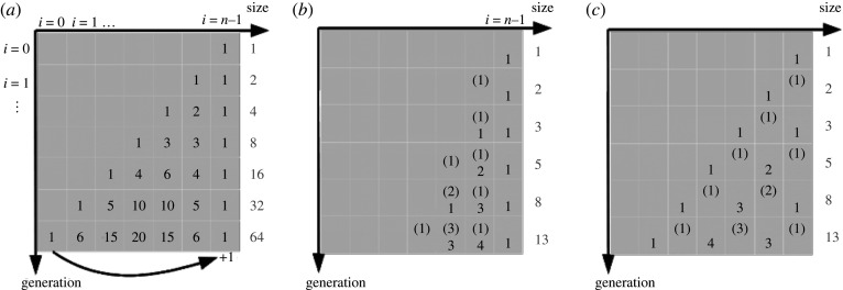
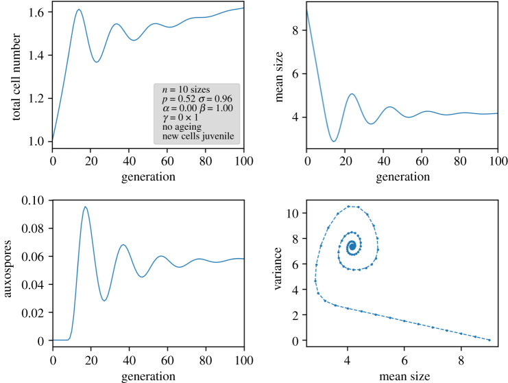
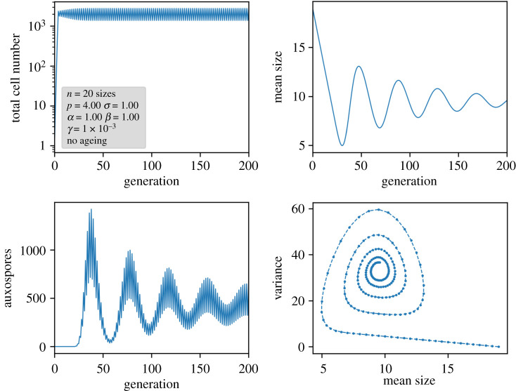
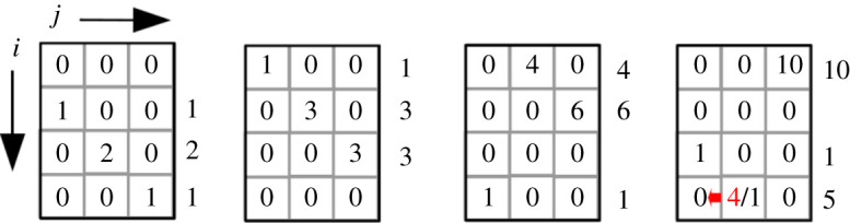
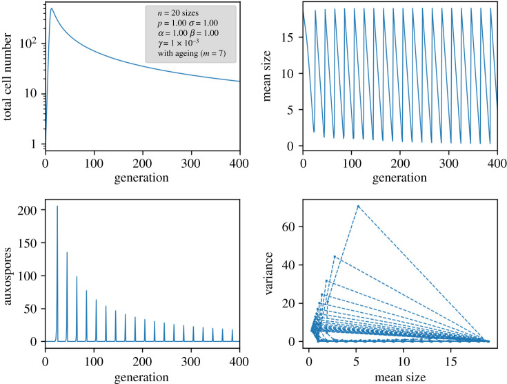
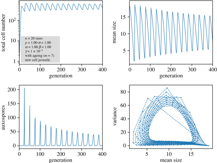
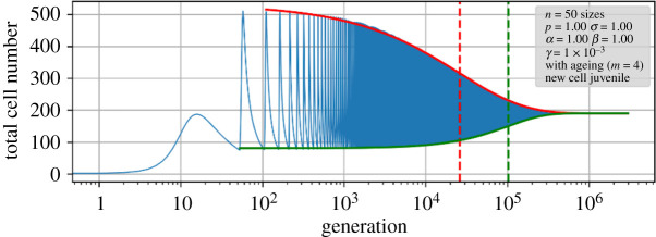
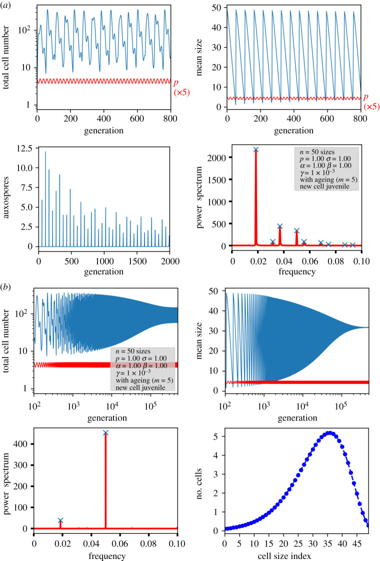
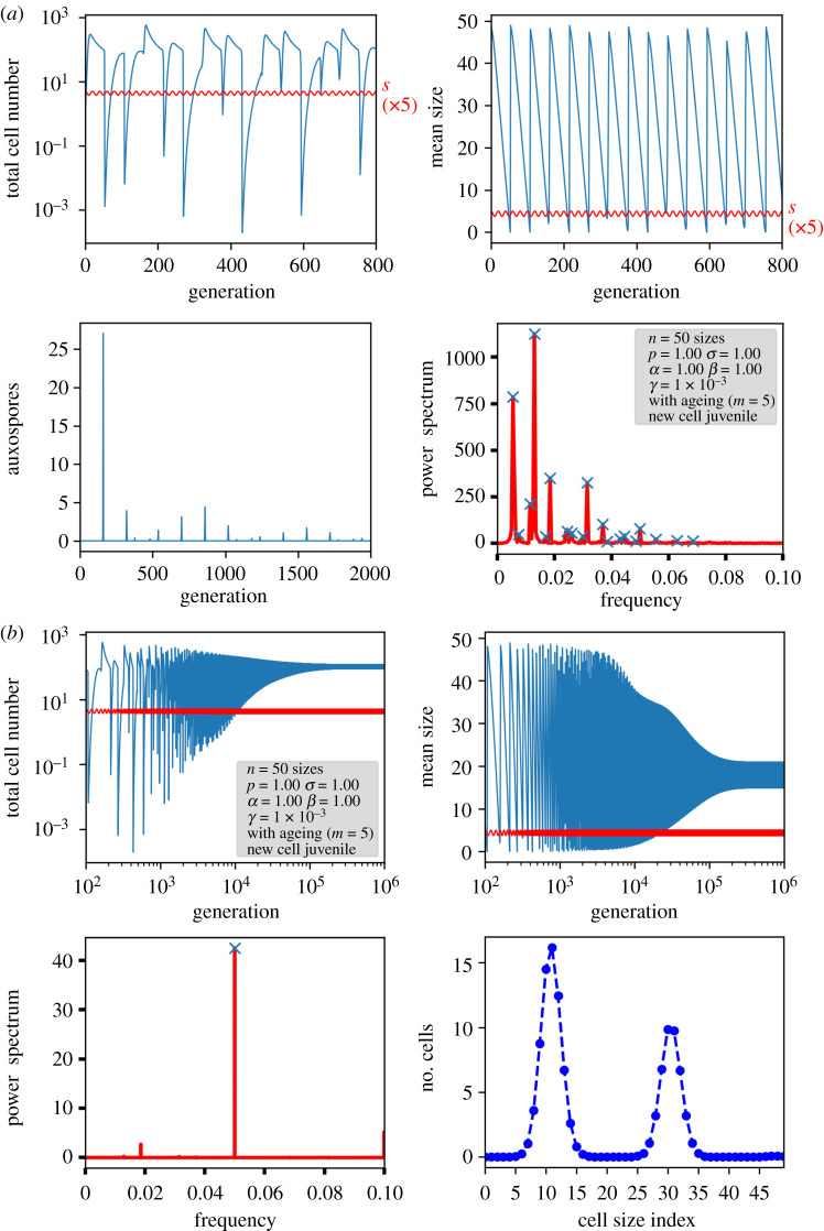
The unique life cycle of diatoms with continuous decreasing and restoration of the cell size leads to periodic fluctuations in cell size distribution and has been regarded as a multi-annual clock. To understand the long-term behaviour of a population analytically, generic mathematical models are investigated algebraically and numerically for their capability to describe periodic oscillations. Whereas the generally accepted simple concepts for the proliferation dynamics do not sustain oscillating behaviour owing to broadening of the size distribution, simulations show that a proposed limited lifetime of a newly synthesized cell wall slows down the relaxation towards a time-invariant equilibrium state to the order of a hundred thousand generations. In combination with seasonal perturbation events, the proliferation scheme with limited lifetime is able to explain long-lasting rhythms that are characteristic for diatom population dynamics. The life cycle thus resembles a pendulum clock that has to be wound up from time to time by seasonal perturbations rather than an oscillator represented by a limit cycle.
Keywords: clocks; diatoms; discrete models; matrix models; oscillations.
Figures
Similar articles
-
bHLH-PAS protein RITMO1 regulates diel biological rhythms in the marine diatom Phaeodactylum tricornutum.Proc Natl Acad Sci U S A. 2019 Jun 25;116(26):13137-13142. doi: 10.1073/pnas.1819660116. Epub 2019 Jun 6. Proc Natl Acad Sci U S A. 2019. PMID: 31171659 Free PMC article.
-
Stochastic models for circadian rhythms: effect of molecular noise on periodic and chaotic behaviour.C R Biol. 2003 Feb;326(2):189-203. doi: 10.1016/s1631-0691(03)00016-7. C R Biol. 2003. PMID: 12754937 Review.
-
Diurnal transcript profiling of the diatom Seminavis robusta reveals adaptations to a benthic lifestyle.Plant J. 2021 Jul;107(1):315-336. doi: 10.1111/tpj.15291. Epub 2021 May 18. Plant J. 2021. PMID: 33901335
-
The brown clock: circadian rhythms in stramenopiles.Physiol Plant. 2020 Jul;169(3):430-441. doi: 10.1111/ppl.13104. Epub 2020 May 4. Physiol Plant. 2020. PMID: 32274814 Review.
-
Biological timing and the clock metaphor: oscillatory and hourglass mechanisms.Chronobiol Int. 2001 May;18(3):329-69. doi: 10.1081/cbi-100103961. Chronobiol Int. 2001. PMID: 11475408 Review.
References
-
- Tréguer P, et al. 2018 Influence of diatom diversity on the ocean biological carbon pump. Nat. Geosci. 11, 27-37. (10.1038/s41561-017-0028-x) - DOI
-
- Nelson DM, Tréguer P, Brzezinski MA, Leynaert A, Quéguiner B. 1995. Production and dissolution of biogenic silica in the ocean: revised global estimates, comparison with regional data and relationship to biogenic sedimentation. Global Biogeochem. Cycles 9, 359-372. (10.1029/95GB01070) - DOI
-
- Smayda TJ. 1997. What is a bloom? A commentary. Limnol. Oceanogr. 42, 1132-1136. (10.4319/lo.1997.42.5_part_2.1132) - DOI
-
- Platt T, White GN, Thai L, Sathyendranath S, Roy S. 2009. The phenology of phytoplankton blooms: ecosystem indicators from remote sensing. Ecol. Model. 220, 3057-3069. (10.1016/j.ecolmodel.2008.11.022) - DOI
Publication types
MeSH terms
Associated data
LinkOut - more resources
Full Text Sources