. 2021 Apr 8:10:e60563.
doi: 10.7554/eLife.60563.

Neural signatures of vigilance decrements predict behavioural errors before they occur

Affiliations

Neural signatures of vigilance decrements predict behavioural errors before they occur

Hamid Karimi-Rouzbahani et al. Elife. .

Erratum in

Abstract

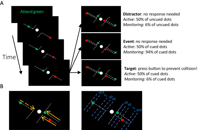
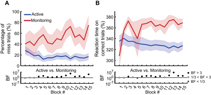
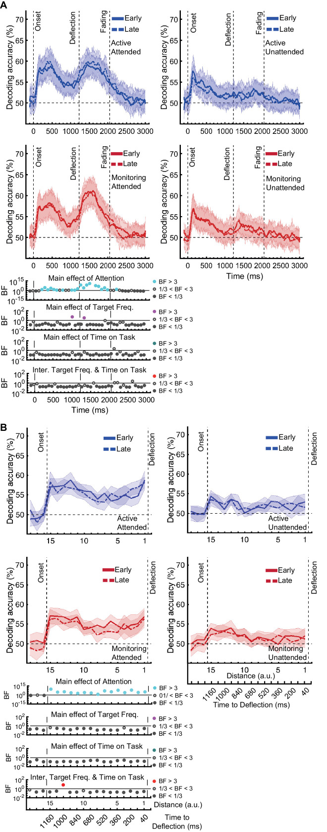
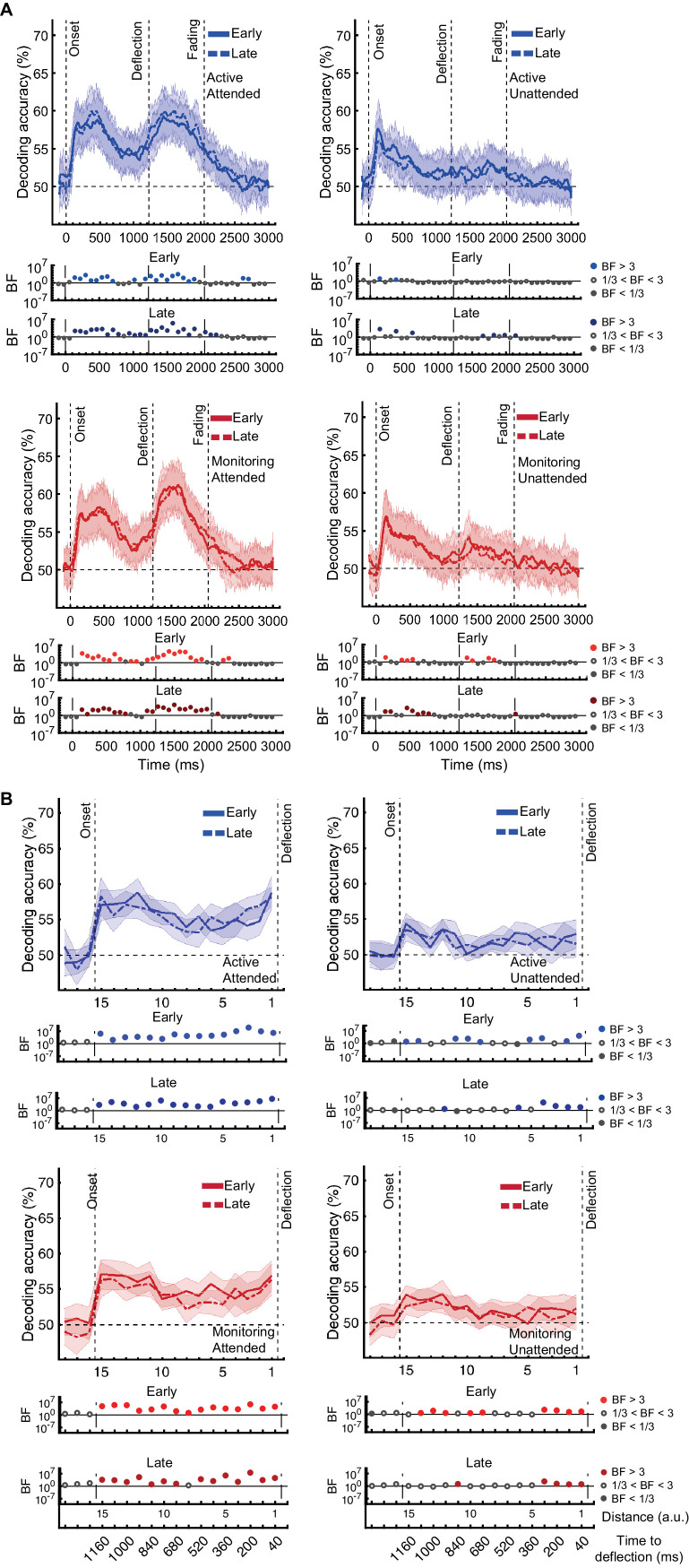
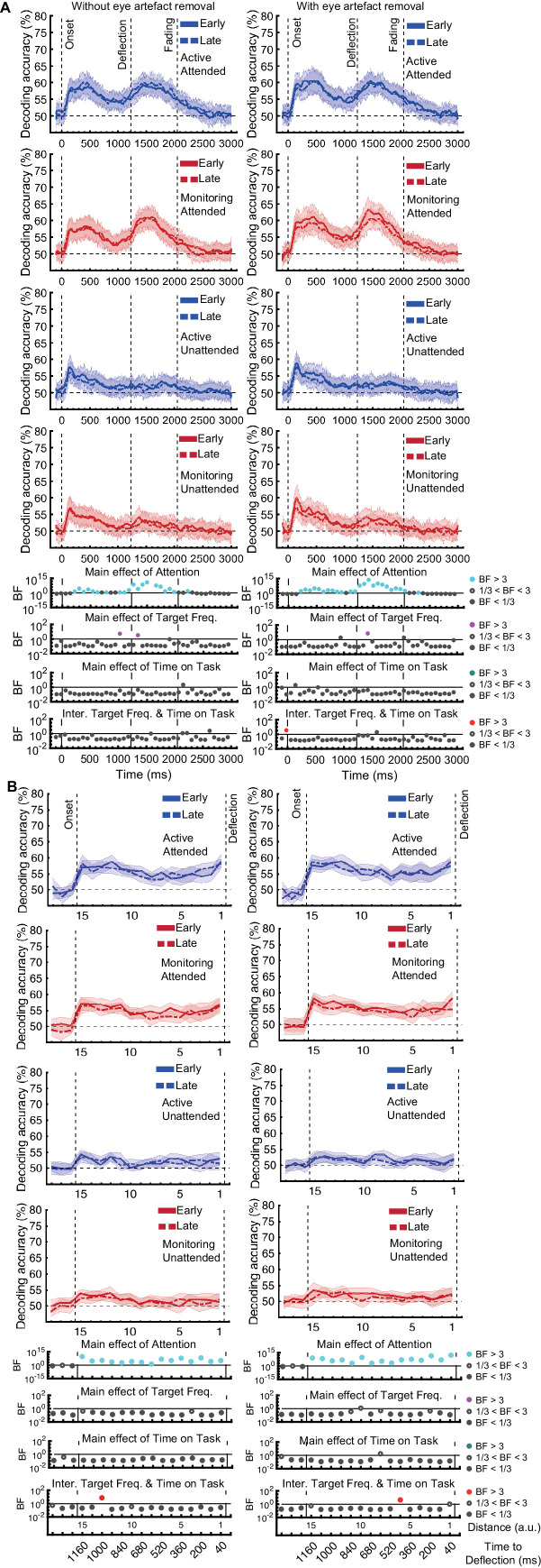
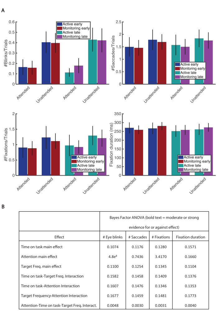
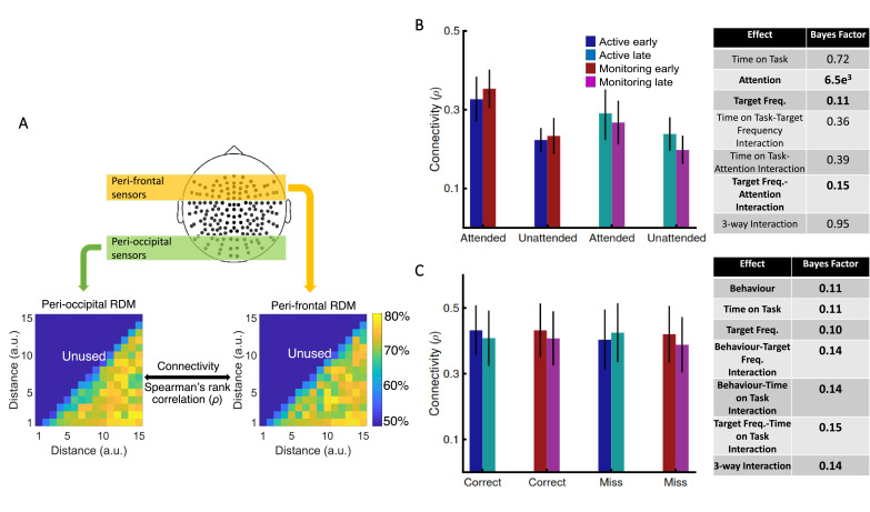
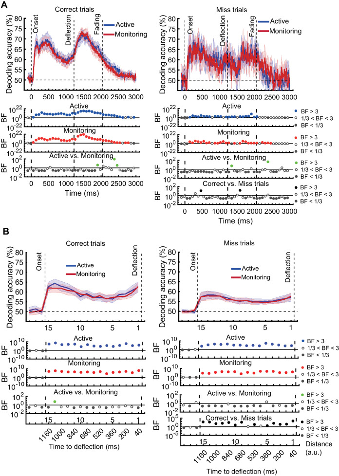
There are many monitoring environments, such as railway control, in which lapses of attention can have tragic consequences. Problematically, sustained monitoring for rare targets is difficult, with more misses and longer reaction times over time. What changes in the brain underpin these 'vigilance decrements'? We designed a multiple-object monitoring (MOM) paradigm to examine how the neural representation of information varied with target frequency and time performing the task. Behavioural performance decreased over time for the rare target (monitoring) condition, but not for a frequent target (active) condition. This was mirrored in neural decoding using magnetoencephalography: coding of critical information declined more during monitoring versus active conditions along the experiment. We developed new analyses that can predict behavioural errors from the neural data more than a second before they occurred. This facilitates pre-empting behavioural errors due to lapses in attention and provides new insight into the neural correlates of vigilance decrements.

Keywords: error prediction; human; informational connectivity; magnetoencephalography; multi-variate pattern analysis; neuroscience; vigilance decrements; visual attention.


Conflict of interest statement

HK, AW, AR No competing interests declared

Figures

Figure 1.
Figure 1.. The multiple-object monitoring (MOM) task and types of information decoded.
(A) At the start of a block, the relevant colour is cued (here, green; distractors in red). Over the on-task period (~30 min per task condition), multiple dots entered from either direction, each moving along a visible individual trajectory towards the middle object. Only attended dots that failed to deflect along the trajectories at the deflection point required a response (Target: bottom right display). Participants did not need to press the button for the unattended dot (Distractor: top right display) or the dots that kept moving on the trajectories (Event: middle right panel). Each dot took ~1226 ms from appearance to deflection. (B) Direction of approach information (left display: left vs. right as indicated by dashed and solid lines, respectively) and distance to object information (right display). Note the blue dashed lines and orange arrows were not present in the actual display. d1, d2, etc. denote the ‘distance units’ used to train the classifier for the key distance to object information. A demo of the task can be found here [https://osf.io/5aw8v/].
Figure 2.
Figure 2.. Behavioural performance on the MOM task.
The percentage of miss trials (A), and correct reaction times (B), as a function of block. Thick lines show the average across participants (shading 95% confidence intervals) for Active (blue) and Monitoring (red) conditions. Each block lasted for 110 s and had either 16 (Active) or 2 (Monitoring) targets out of 32 cued-colour and 32 non-cued colour dots. Bayes factors (BF) are shown in the bottom section of each graph: Filled circles show moderate/strong evidence for either hypothesis and empty circles indicate insufficient evidence when evaluating the contrast between Active and Monitoring conditions.
Figure 3.
Figure 3.. Impact of different conditions and their interactions on information on correct trials (all trials except those in which a target was missed or there was a false alarm).
(A) Decoding of direction of approach information (less task-relevant) and (B) decoding of distance to object information (most task-relevant). Left two columns: Attended dots; Right two columns: Unattended (‘distractor’) dots. Thick lines show the average across participants (shading 95% confidence intervals). Horizontal dashed line refers to theoretical chance-level decoding (50%). Vertical dashed lines indicate critical times in the trial. Bottom panels: Bayesian evidence for main effects and interactions, Bayes factors (BF): Filled circles show moderate/strong evidence for either hypothesis and empty circles indicate insufficient evidence. Main effects and interactions of conditions calculated using BF ANOVA analysis. Cyan, purple, green, and red dots indicate the main effects of Attention, Target frequency, Time on Task, and the interaction between Target frequency and Time on Task, respectively. The results of BF analysis (i.e., the main effects of the three conditions and their interactions) are from the same three-way ANOVA analysis and are therefore identical for attended and unattended panels. Early = data from the first five blocks (~10 min). Late = data from the last five blocks (~10 min). Note the different scales of the BF panels, and the down-sampling, for clearer illustration.
Figure 3—figure supplement 1.
Figure 3—figure supplement 1.. Impact of different conditions in the direction of approach and distance to object information coding and their Bayesian evidence for difference from chance.
Two left graphs: Attended dots; Two right graphs: Unattended (‘distractor’) dots. (A) Decoding of direction of approach information (less task-relevant). (B) Decoding of distance to object information (most task-relevant). Thick lines show the average across participants (shading 95% confidence intervals). The horizontal dashed lines refer to chance-level decoding. Vertical dashed lines indicate critical times in the trial. Bayes factors (BF) are shown in the bottom section of each graph: Filled circles show moderate/strong evidence for either hypothesis and empty circles indicate insufficient evidence. They show the results of BF analysis when evaluating the difference of the decoding values from chance as explained in Materials and methods. Early = data from the first five blocks (~10 min). Late = data from the last five blocks (~10 min). Note the different scales of the BF panels, and the down-sampling, for clearer illustration.
Figure 3—figure supplement 2.
Figure 3—figure supplement 2.. Impact of different conditions and their interactions on information processing on correct trials (all trials except those in which a target was missed or there was a false alarm) without and with standard eye-artefact removal.
Left and right panels show the results without (repeated from Figure 3) and with eye-standard eye-artefact removal, respectively. (A) Decoding of direction of approach information (less task-relevant) and (B) decoding of distance to object information (most task-relevant). Left two columns: Attended dots; Right two columns: Unattended (‘distractor’) dots. Thick lines show the average across participants (shading 95% confidence intervals). Horizontal dashed line refers to theoretical chance-level decoding (50%). Vertical dashed lines indicate critical times in the trial. Bottom panels: Bayesian evidence for main effects and interactions, Bayes factors (BF): Filled circles show moderate/strong evidence for either hypothesis and empty circles indicate insufficient evidence. Main effects and interactions of conditions calculated using BF ANOVA analysis. Cyan, purple, green, and red dots indicate the main effects of Attention, Target frequency, Time on Task, and the interaction between Target frequency and Time on Task, respectively. The results of BF analysis (i.e., the main effects of the three conditions and their interactions) are from the same three-way ANOVA analysis and are therefore identical for attended and unattended panels. Early = data from the first five blocks (~10 min). Late = data from the last five blocks (~10 min). Note the different scales of the BF panels, and the down-sampling, for clearer illustration.
Figure 3—figure supplement 3.
Figure 3—figure supplement 3.. The statistical relationship between the proportion of eye-related measures and Target Frequency, Attention, and Time on the task factors.
(A) Eye-related measures. The error bars show 95% confidence interval around the mean across participants. (B) Bayes factor evidence for the main effects and interactions between factors and eye-related measures.
Figure 4.
Figure 4.. Relationship between informational connectivity and Attention, Target Frequency, Time on Task, and the behavioural outcome of the trial (i.e., correct vs. miss).
(A) Calculation of connectivity using Spearman’s rank correlation between RDMs obtained from the peri-frontal and peri-occipital sensors as indicated by coloured boxes, respectively. RDMs include decoding accuracies obtained from testing the 105 classifiers trained to discriminate different distance to object categories. (B) Connectivity values for the eight different conditions of the task and the results of three-way Bayes factor ANOVA with factors Time on Task (Early, Late), Attention (Attended, Unattended), and Target Frequency (Active, Monitoring), using only correct trials. (C) Connectivity values for the Active and Monitoring, Early and Late blocks of each task for correct and miss trials (attended condition only), and the result of Bayes factor ANOVA with factors Target Frequency (Active, Monitoring), Time on Task (Early, Late), and behavioural outcome (correct, miss) as inputs. Number of trials are equalised across conditions in B and C separately. Bars show the average across participants (error bars 95% confidence intervals). Bold fonts indicate moderate or strong evidence for either the effect or the null hypothesis.
Figure 5.
Figure 5.. Decoding of information on correct vs miss trials.
(A) Decoding of direction of approach information (less task-relevant). (B) Decoding of distance to object information (most task-relevant). The horizontal dashed lines refer to theoretical chance-level decoding. Left panels: Decoding using correct trials; Right panels: Decoding using miss trials. In both right and left panels, the classifiers were trained on correct trials and tested on (left out) correct and all miss trials, respectively. Thick lines show the average across participants (shading 95% confidence intervals). Vertical dashed lines indicate critical events in the trial. Bayes factors (BF) are shown in the bottom section of each graph: Filled circles show moderate/strong evidence for either hypothesis and empty circles indicate insufficient evidence. They show the results of BF analysis when evaluating the difference of the decoding values from chance for Active (blue) and Monitoring (red) conditions separately, the comparison of the two conditions (green), and the comparison of correct and miss trials (black). Note that for the comparison of correct and miss trials, Active and Monitoring conditions were averaged separately. Note the different scales of the BF panels, and down-sampling, for clearer illustration.
Figure 5—figure supplement 1.
Figure 5—figure supplement 1.. Distribution of decoding accuracies for every individual correct and miss trial in the Active and Monitoring conditions for all 21 subjects.
A and B show the data for correct and miss trials, respectively. The percentages show the percentage of trials for which there was strong (BF >10) evidence for above-chance decoding in Active and Monitoring conditions. (C) Difference between the decoding accuracies in the correct (A) and miss (B) trials as evaluated using Cohen’s d.
Figure 5—figure supplement 2.
Figure 5—figure supplement 2.. Decoding of information on correct vs false alarm trials.
(A) Decoding of direction of approach information (less task-relevant). (B) Decoding of distance to object information (most task-relevant). The horizontal dashed lines refer to theoretical chance-level decoding. Left panels: Decoding using correct trials; Right panels: Decoding using false alarm trials. In both right and left panels, the classifiers were trained on correct trials and tested on (left out) correct and all false alarm trials, respectively. Thick lines show the average across participants (shading 95% confidence intervals). Vertical dashed lines indicate critical events in the trial. Bayes factors (BF) are shown in the bottom section of each graph: Filled circles show moderate/strong evidence for either hypothesis and empty circles indicate insufficient evidence. They show the results of BF analysis when evaluating the difference of the decoding values from chance for Active (blue) and Monitoring (red) conditions separately, the comparison of the two conditions (green) and the comparison of correct and false alarm trials (black). Note that for the comparison of correct and miss trials, Active and Monitoring conditions were averaged separately. Note the different scales of the BF panels, and the down-sampling, for clearer illustration.
Figure 6.
Figure 6.. Prediction of behavioural outcome (correct vs miss) trial-by-trial using decoding of distance to object information.
(A) Sample classifiers’ accuracies (correct or incorrect classification of current distance as indicated by colours) for a miss (left panel; average accuracy ≅ 43% when the dot reached the deflection point) and a correct trial (right panel; average accuracy ≅ 67% at the deflection point). The classifiers were trained on the data from correct trials and tested on the data from correct and miss trials. For the miss trials, around half the classifiers categorised the dot’s distance incorrectly by the time it reached the deflection point. (B) Accumulation of classifiers’ accuracies over decreasing dot distances/time to deflection. This shows stronger information coding of the crucial distance to object information on the correct trials over miss trials. A variable threshold used in (C) is shown as a green dashed line. (C) Prediction of behavioural outcome as a function of threshold and distance using a second-level behavioural outcome classification. Results showed highest prediction accuracies on the participant set at around the threshold of 0.4SD under the decoding level for correct validation trials, increasing at closer distances. (D) Accuracy of predicting behavioural outcome for the left-out participant using the threshold obtained from all the other participants as function of distance/time from the deflection point. Results showed successful (~=59%) prediction of behavioural outcome of the trial as early as 80 ms after stimulus appearance. Thick lines and shading refer to average and one standard deviation around the mean across participants, respectively. Bayes factors (BF) are shown in the bottom section of each graph: Filled circles show moderate/strong evidence for either hypothesis and empty circles indicate insufficient evidence (black dots under B and D).
Figure 6—figure supplement 1.
Figure 6—figure supplement 1.. Accuracy of predicting behavioural outcome of trials in the early (first 5) vs late (last 5) blocks of trials before eye-blink removal.
Left column shows the result for the early and right shows the result for the late blocks. (A) Result of classifier accumulation of decoding accuracy. (B) Prediction accuracy and (C) same results (as in B) overlapping on the same plot with Bayes factor (BF) analysis of the difference. The details of this figure are identical to Figure 6B and D. BF in A and C show the evidence for and against the alternative of difference between the curves and the BFs in B reflect the evidence for and against the alternative for difference from chance.
Author response image 1.
Author response image 1.. The accuracy of predicting behavioral outcome of trials without and with eye artefact removal.
The results are for the left-out participant (averaged over all participants) using the threshold obtained from all the other participants as function of distance/time from the deflection point. Figure 6D shows the result without eye artefact removal and Author response image 1 with eye artefact removal. Thick lines and shading refer to average and one standard deviation around the mean across participants, respectively. Bayes Factors are shown in the bottom section of each graph: Filled circles show moderate/strong evidence for either hypothesis and empty circles indicate insufficient evidence.

Similar articles

Cited by

References

    1. Adler CM, Sax KW, Holland SK, Schmithorst V, Rosenberg L, Strakowski SM. Changes in neuronal activation with increasing attention demand in healthy volunteers: an fMRI study. Synapse. 2001;42:266–272. doi: 10.1002/syn.1112. - DOI - PubMed
    1. Alnæs D, Kaufmann T, Richard G, Duff EP, Sneve MH, Endestad T, Nordvik JE, Andreassen OA, Smith SM, Westlye LT. Attentional load modulates large-scale functional brain connectivity beyond the core attention networks. NeuroImage. 2015;109:260–272. doi: 10.1016/j.neuroimage.2015.01.026. - DOI - PubMed
    1. Anzellotti S, Coutanche MN. Beyond functional connectivity: investigating networks of multivariate representations. Trends in Cognitive Sciences. 2018;22:258–269. doi: 10.1016/j.tics.2017.12.002. - DOI - PubMed
    1. Baillet S. Magnetoencephalography for brain electrophysiology and imaging. Nature Neuroscience. 2017;20:327–339. doi: 10.1038/nn.4504. - DOI - PubMed
    1. Basti A, Nili H, Hauk O, Marzetti L, Henson RN. Multi-dimensional connectivity: a conceptual and mathematical review. NeuroImage. 2020;221:117179. doi: 10.1016/j.neuroimage.2020.117179. - DOI - PubMed

Publication types

LinkOut - more resources