

Targeted realignment of LC-MS profiles by neighbor-wise compound-specific graphical time warping with misalignment detection
- PMID: 31950989
- PMCID: PMC7203744
- DOI: 10.1093/bioinformatics/btaa037
Targeted realignment of LC-MS profiles by neighbor-wise compound-specific graphical time warping with misalignment detection
Abstract
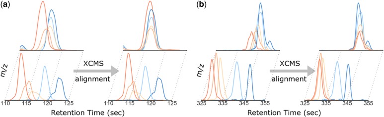
Motivation: Liquid chromatography-mass spectrometry (LC-MS) is a standard method for proteomics and metabolomics analysis of biological samples. Unfortunately, it suffers from various changes in the retention times (RT) of the same compound in different samples, and these must be subsequently corrected (aligned) during data processing. Classic alignment methods such as in the popular XCMS package often assume a single time-warping function for each sample. Thus, the potentially varying RT drift for compounds with different masses in a sample is neglected in these methods. Moreover, the systematic change in RT drift across run order is often not considered by alignment algorithms. Therefore, these methods cannot effectively correct all misalignments. For a large-scale experiment involving many samples, the existence of misalignment becomes inevitable and concerning.
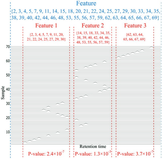
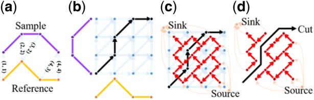
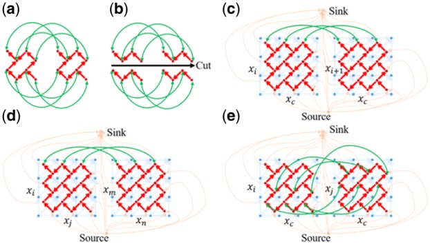
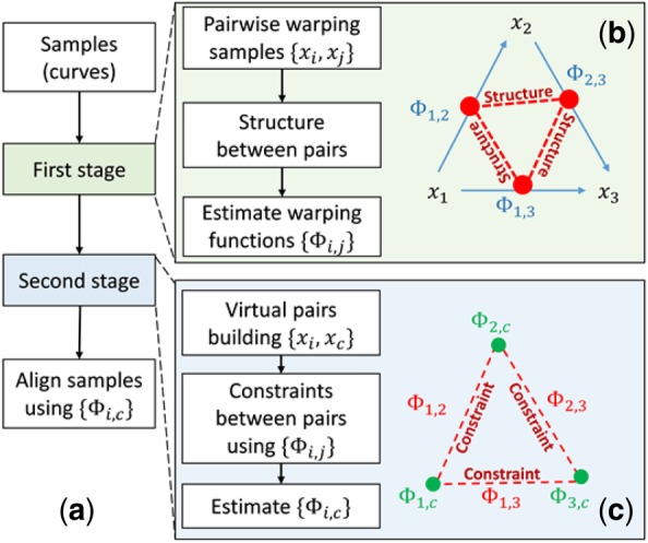
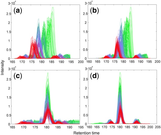
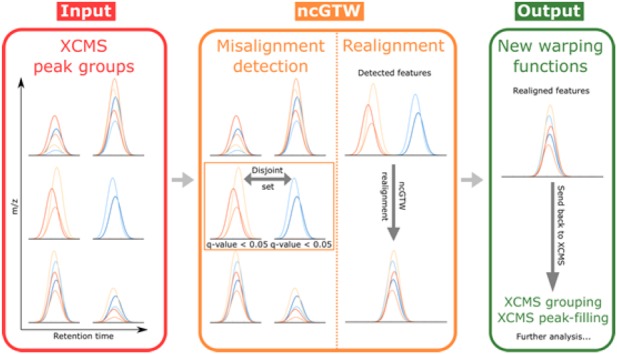
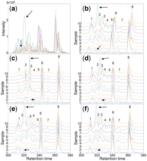
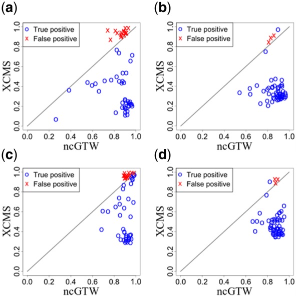
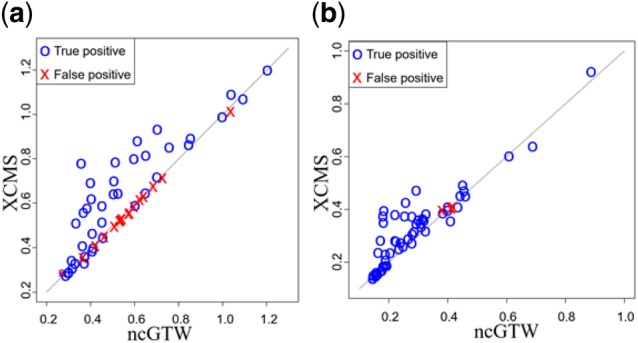
Results: Here, we describe an integrated reference-free profile alignment method, neighbor-wise compound-specific Graphical Time Warping (ncGTW), that can detect misaligned features and align profiles by leveraging expected RT drift structures and compound-specific warping functions. Specifically, ncGTW uses individualized warping functions for different compounds and assigns constraint edges on warping functions of neighboring samples. Validated with both realistic synthetic data and internal quality control samples, ncGTW applied to two large-scale metabolomics LC-MS datasets identifies many misaligned features and successfully realigns them. These features would otherwise be discarded or uncorrected using existing methods. The ncGTW software tool is developed currently as a plug-in to detect and realign misaligned features present in standard XCMS output.
Availability and implementation: An R package of ncGTW is freely available at Bioconductor and https://github.com/ChiungTingWu/ncGTW. A detailed user's manual and a vignette are provided within the package.
Supplementary information: Supplementary data are available at Bioinformatics online.
© The Author(s) 2020. Published by Oxford University Press. All rights reserved. For permissions, please e-mail: journals.permissions@oup.com.
Figures
Similar articles
-
MetTailor: dynamic block summary and intensity normalization for robust analysis of mass spectrometry data in metabolomics.Bioinformatics. 2015 Nov 15;31(22):3645-52. doi: 10.1093/bioinformatics/btv434. Epub 2015 Jul 27. Bioinformatics. 2015. PMID: 26220962
-
G-Aligner: a graph-based feature alignment method for untargeted LC-MS-based metabolomics.BMC Bioinformatics. 2023 Nov 14;24(1):431. doi: 10.1186/s12859-023-05525-4. BMC Bioinformatics. 2023. PMID: 37964228 Free PMC article.
-
Time alignment algorithms based on selected mass traces for complex LC-MS data.J Proteome Res. 2010 Mar 5;9(3):1483-95. doi: 10.1021/pr9010124. J Proteome Res. 2010. PMID: 20070124
-
Translational Metabolomics of Head Injury: Exploring Dysfunctional Cerebral Metabolism with Ex Vivo NMR Spectroscopy-Based Metabolite Quantification.In: Kobeissy FH, editor. Brain Neurotrauma: Molecular, Neuropsychological, and Rehabilitation Aspects. Boca Raton (FL): CRC Press/Taylor & Francis; 2015. Chapter 25. In: Kobeissy FH, editor. Brain Neurotrauma: Molecular, Neuropsychological, and Rehabilitation Aspects. Boca Raton (FL): CRC Press/Taylor & Francis; 2015. Chapter 25. PMID: 26269925 Free Books & Documents. Review.
-
Tutorial: Correction of shifts in single-stage LC-MS(/MS) data.Anal Chim Acta. 2018 Jan 25;999:37-53. doi: 10.1016/j.aca.2017.09.039. Epub 2017 Nov 2. Anal Chim Acta. 2018. PMID: 29254573 Review.
Cited by
-
Alignment of multiple metabolomics LC-MS datasets from disparate diseases to reveal fever-associated metabolites.PLoS Negl Trop Dis. 2023 Jul 24;17(7):e0011133. doi: 10.1371/journal.pntd.0011133. eCollection 2023 Jul. PLoS Negl Trop Dis. 2023. PMID: 37486920 Free PMC article.
-
Finding Correspondence between Metabolomic Features in Untargeted Liquid Chromatography-Mass Spectrometry Metabolomics Datasets.Anal Chem. 2022 Apr 12;94(14):5493-5503. doi: 10.1021/acs.analchem.1c03592. Epub 2022 Mar 31. Anal Chem. 2022. PMID: 35360896 Free PMC article.
-
Alignstein: Optimal transport for improved LC-MS retention time alignment.Gigascience. 2022 Nov 3;11:giac101. doi: 10.1093/gigascience/giac101. Gigascience. 2022. PMID: 36329619 Free PMC article.
-
New software tools, databases, and resources in metabolomics: updates from 2020.Metabolomics. 2021 May 11;17(5):49. doi: 10.1007/s11306-021-01796-1. Metabolomics. 2021. PMID: 33977389 Free PMC article. Review.
-
metabCombiner 2.0: Disparate Multi-Dataset Feature Alignment for LC-MS Metabolomics.Metabolites. 2024 Feb 15;14(2):125. doi: 10.3390/metabo14020125. Metabolites. 2024. PMID: 38393017 Free PMC article.
References
-
- Arnold B.C. et al. (1992) A First Course in Order Statistics. Siam, Philadelphia, PA.
-
- Benk A.S., Roesli C. (2012) Label-free quantification using MALDI mass spectrometry: considerations and perspectives. Anal. Bioanal. Chem., 404, 1039–1056. - PubMed
-
- Bild D.E. et al. (2002) Multi-ethnic study of atherosclerosis: objectives and design. Am. J. Epidemiol., 156, 871–881. - PubMed
-
- Christin C. et al. (2008) Optimized time alignment algorithm for LC−MS data: correlation optimized warping using component detection algorithm-selected mass chromatograms. Anal. Chem., 80, 7012–7021. - PubMed
-
- Goldberg A.V. et al. (2011) Maximum flows by incremental breadth-first search In: European Symposium on Algorithms. Springer, Berlin, Heidelberg, pp. 457–468.
