

Diversity in biology: definitions, quantification and models
- PMID: 31899899
- PMCID: PMC8788892
- DOI: 10.1088/1478-3975/ab6754
Diversity in biology: definitions, quantification and models
Abstract
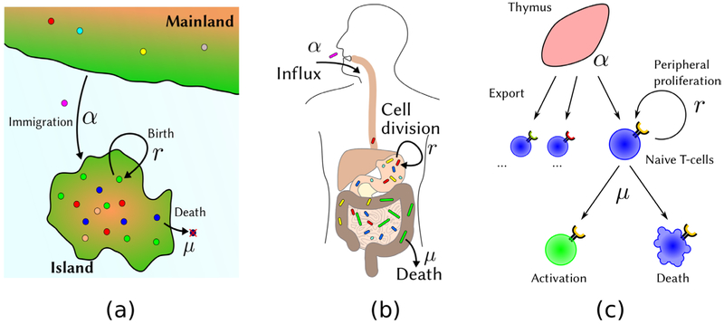
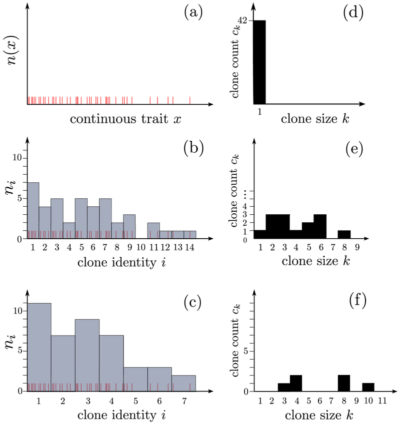
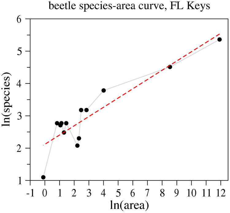
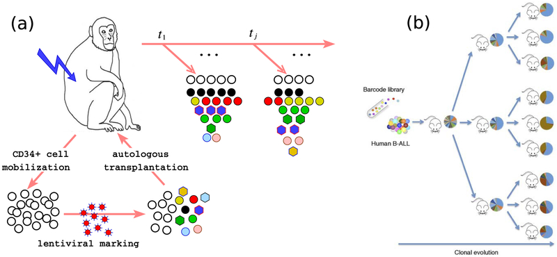
Diversity indices are useful single-number metrics for characterizing a complex distribution of a set of attributes across a population of interest. The utility of these different metrics or sets of metrics depends on the context and application, and whether a predictive mechanistic model exists. In this topical review, we first summarize the relevant mathematical principles underlying heterogeneity in a large population, before outlining the various definitions of 'diversity' and providing examples of scientific topics in which its quantification plays an important role. We then review how diversity has been a ubiquitous concept across multiple fields, including ecology, immunology, cellular barcoding experiments, and socioeconomic studies. Since many of these applications involve sampling of populations, we also review how diversity in small samples is related to the diversity in the entire population. Features that arise in each of these applications are highlighted.
Figures


Similar articles
-
Acoustic indices as proxies for biodiversity: a meta-analysis.Biol Rev Camb Philos Soc. 2022 Dec;97(6):2209-2236. doi: 10.1111/brv.12890. Epub 2022 Aug 17. Biol Rev Camb Philos Soc. 2022. PMID: 35978471 Free PMC article. Review.
-
Translational Metabolomics of Head Injury: Exploring Dysfunctional Cerebral Metabolism with Ex Vivo NMR Spectroscopy-Based Metabolite Quantification.In: Kobeissy FH, editor. Brain Neurotrauma: Molecular, Neuropsychological, and Rehabilitation Aspects. Boca Raton (FL): CRC Press/Taylor & Francis; 2015. Chapter 25. In: Kobeissy FH, editor. Brain Neurotrauma: Molecular, Neuropsychological, and Rehabilitation Aspects. Boca Raton (FL): CRC Press/Taylor & Francis; 2015. Chapter 25. PMID: 26269925 Free Books & Documents. Review.
-
Diversity from genes to ecosystems: A unifying framework to study variation across biological metrics and scales.Evol Appl. 2018 Feb 20;11(7):1176-1193. doi: 10.1111/eva.12593. eCollection 2018 Aug. Evol Appl. 2018. PMID: 30026805 Free PMC article.
-
Measuring diversity from dissimilarities with Rao's quadratic entropy: are any dissimilarities suitable?Theor Popul Biol. 2005 Jun;67(4):231-9. doi: 10.1016/j.tpb.2005.01.004. Theor Popul Biol. 2005. PMID: 15888302
-
Mathematical bounds on Shannon entropy given the abundance of the ith most abundant taxon.J Math Biol. 2023 Oct 26;87(5):76. doi: 10.1007/s00285-023-01997-3. J Math Biol. 2023. PMID: 37884812 Free PMC article.
Cited by
-
Leveraging Experimental Strategies to Capture Different Dimensions of Microbial Interactions.Front Microbiol. 2021 Sep 27;12:700752. doi: 10.3389/fmicb.2021.700752. eCollection 2021. Front Microbiol. 2021. PMID: 34646243 Free PMC article. Review.
-
Surrogate modeling and control of medical digital twins.ArXiv [Preprint]. 2024 May 20:arXiv:2402.05750v2. ArXiv. 2024. Update in: PLoS Comput Biol. 2025 Jan 14;21(1):e1012138. doi: 10.1371/journal.pcbi.1012138. PMID: 38827450 Free PMC article. Updated. Preprint.
-
Quantifying information of intracellular signaling: progress with machine learning.Rep Prog Phys. 2022 Jul 12;85(8):10.1088/1361-6633/ac7a4a. doi: 10.1088/1361-6633/ac7a4a. Rep Prog Phys. 2022. PMID: 35724636 Free PMC article. Review.
-
Clonal dominance in excitable cell networks.Nat Phys. 2021 Dec;17(12):1391-1395. doi: 10.1038/s41567-021-01383-0. Epub 2021 Nov 1. Nat Phys. 2021. PMID: 35242199 Free PMC article.
-
Chaotic turnover of rare and abundant species in a strongly interacting model community.Proc Natl Acad Sci U S A. 2024 Mar 12;121(11):e2312822121. doi: 10.1073/pnas.2312822121. Epub 2024 Mar 4. Proc Natl Acad Sci U S A. 2024. PMID: 38437535 Free PMC article.
References
-
- Heywood VH et al. 1995. Global Biodiversity Assessment vol 1140 (Cambridge: Cambridge University Press; )
-
- Purvis A and Hector A 2000. Getting the measure of biodiversity Nature 405 212. - PubMed
-
- Whittaker RJ, Willis KJ and Field R 2001. Scale and species richness: towards a general, hierarchical theory of species diversity J. Biogeogr 28 453–70
-
- Sala OE et al. 2000. Global biodiversity scenarios for the year 2100 Science 287 1770–4 - PubMed