. 2019 Apr;127(4):47004.
doi: 10.1289/EHP3711.

Associations between High Temperature, Heavy Rainfall, and Diarrhea among Young Children in Rural Tamil Nadu, India: A Prospective Cohort Study

Affiliations

Associations between High Temperature, Heavy Rainfall, and Diarrhea among Young Children in Rural Tamil Nadu, India: A Prospective Cohort Study

Andrew Mertens et al. Environ Health Perspect. 2019 Apr.

Abstract

Background: The effects of weather on diarrhea could influence the health impacts of climate change. Children have the highest diarrhea incidence, especially in India, where many lack safe water and sanitation.

Objectives: In a prospective cohort of 1,284 children under 5 y of age from 900 households across 25 villages in rural Tamil Nadu, India, we examined whether high temperature and heavy rainfall was associated with increased all-cause diarrhea and water contamination.

Methods: Seven-day prevalence of diarrhea was assessed monthly for up to 12 visits from January 2008 to April 2009, and hydrogen sulfide ([Formula: see text]) presence in drinking water, a fecal contamination indicator, was tested in a subset of households. We estimated associations between temperature and rainfall exposures and diarrhea and [Formula: see text] using binomial regressions, adjusting for potential confounders, random effects for village, and autoregressive-1 error terms for study week.

Results: There were 259 cases of diarrhea. The prevalence of diarrhea during the 7 d before visits was 2.95 times higher (95% CI: 1.99, 4.39) when mean temperature in the week before the 7-d recall was in the hottest versus the coolest quartile of weekly mean temperature during 1 December 2007 to 15 April 2009. Diarrhea prevalence was 1.50 times higher when the 3 weeks before the diarrhea recall period included [Formula: see text] (vs. 0 d) with rainfall of [Formula: see text] (95% CI: 1.12, 2.02), and 2.60 times higher (95% CI: 1.55, 4.36) for heavy rain weeks following a 60-d dry period. The [Formula: see text] prevalence in household water was not associated with heavy rain prior to sample collection.

Conclusions: The results suggest that, in rural Tamil Nadu, heavy rainfall may wash pathogens that accumulate during dry weather into child contact. Higher temperatures were positively associated with diarrhea 1-3 weeks later. Our findings suggest that diarrhea morbidity could worsen under climate change without interventions to reduce enteric pathogen transmission through multiple pathways. https://doi.org/10.1289/EHP3711.


Figures
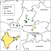
Figure 1 is a part of a map of Tamil Nadu, marking the airport weather station and the control and intervention villages in Tiruchirappalli. An outline map of India and the legend of the intervention statuses are inset.
Figure 1.
Map of study region with points marking the location of airport weather station and the intervention and control villages. The map shows the study area in the Tiruchirappalli region in southern India, with study villages plotted as points. The red box in the inset map of India shows where the study region was located within India, and the points are colored dark green for villages receiving the combination of WASH interventions and light yellow for matched control villages. The X-marked point indicates the location of the Tiruchirappalli Airport weather station, where rainfall and temperature were measured over the study period (1 December 2007 to 15 April 2009) and assumed to generalize to all the study villages.
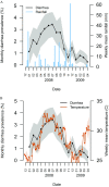
Figures 2A and 2B are graphs plotting monthly diarrhea prevalence ranging between 0 and 5 percentage (left y-axis) and weekly mean rainfall ranging between 0 to 60 millimeters and weekly mean temperature ranging between 25 to 35 Celsius (right y-axis), respectively, across specific dates during the years 2008 and 2009.
Figure 2.
Diarrhea prevalence, rainfall, and temperature over the study period. (A) Mean 7-d prevalence of diarrhea during each month [with 95% confidence interval (CI) band] and weekly rain accumulation over the study period (December 2007–April 2009). (B) Mean 7-d prevalence of diarrhea during each month (with 95% CI band) and weekly mean temperature over the study period.
Figure 3A consists of three graphs showing cubic splines for one week lag, two week lag, and three week lag, plotting diarrhea prevalence ranging between 0 and 6 percentage (y-axis) across weekly mean temperature ranging between 24 and 34 Celsius (x-axis). Figure 3B consists of three graphs plotting comparisons of prevalence ratios of diarrhea associations ranging between 0.50 and 8.00 (y-axis) for one week lag, two week lag, and three week lag, across quartiles of weekly mean temperature ranging between Q1 and Q4 (x-axis). Figure 3C consists of three graphs plotting comparisons of prevalence ratios of drinking water associations ranging between 0.75 and 1.33 (y-axis) for one week lag, two week lag, and three week lag, across quartiles of weekly mean temperature ranging between Q1 and Q4 (x-axis).
Figure 3.
Relationships between weekly mean temperature and 7-d prevalence of diarrhea among children 5 in and H2S in stored household drinking water 1, 2, or 3 weeks prior to the 7-d diarrhea recall period, Tamil Nadu, India, 2008–2009. (A) Adjusted associations between weekly temperature and the 7-d prevalence of diarrhea (95% simultaneous confidence bands) estimated with cubic splines, fit with 3 df. The vertical dashed lines in the temperature plots mark the 25th, 50th, and 75th percentiles of temperature over the study period. Observed diarrhea cases are plotted as points at the top of each plot and observed noncases are plotted as points at the bottom of each graph. Points are jittered for visibility. The weekly mean temperature is lagged 1 (left panel), 2 (middle panel), and 3 weeks (right panel) prior to the start of the 7-d diarrhea recall period. (B) Adjusted prevalence ratios (with 95% CI) for diarrhea according to quartiles (Q) of weekly mean temperature lagged 1, 2, and 3 weeks prior to the start of the 7-d diarrhea recall period. Q1–Q4 indicate mean weekly temperature quartiles 1–4, with the first (lowest) quartile of temperature used as the reference level to calculate prevalence ratios, and using 26.1, 28.1, and 30.5°C as the cutoffs between the quartiles. Prevalence ratios were estimated with binomial regressions (log-link) models that included random effects for village membership and an autoregressive-1 error term on the study week of the household visit and potential confounders selected via likelihood ratio tests. The selected covariates were child age; intervention group; primary water source; current breastfeeding status; indicators for household participation in a community group, credit finance group, or agriculture; indicators for if the household had electricity, a thatched roof, a bank account, or a dirt floor; indicators for presence of water, soap, ash, towel/cloth, sink, or flies at the household handwashing station; indicators for ownership of a dog or cat, ox, television, motorcycle or scooter, or mosquito net; and indicator for reported open defecation from a household member. The model with a 3-week lag period was additionally adjusted for mean weekly rainfall during the week of temperature exposure. (See Table S1 for numeric data.) (C) Adjusted prevalence ratios (with 95% CI) for the presence of H2S in household stored drinking-water samples according to quartiles of weekly mean temperature lagged 1, 2, and 3 weeks prior to the start of the 7-d diarrhea recall period. Q1–Q4 indicate mean weekly temperature quartiles 1–4, with the first (lowest) quartile of temperature used as the reference level to calculate prevalence ratios, and using 26.1, 28.1, and 30.5°C as the cutoffs between the quartiles. Prevalence ratios were estimated with binomial regressions (log-link) models that included random effects for village membership and an autoregressive-1 error term on the study week of the household visit and potential confounders selected via likelihood ratio tests. The selected covariates were mean weekly rainfall during the week of temperature exposure; child sex; intervention group; primary water source; maternal age and education; indicators for presence of soap, ash, or sink at the household handwashing station; indicators for if the household has a bank account, a ventilated kitchen, or a latrine; primary cooking fuel used; family-owned land; family-owned home; indicator for if family is from a scheduled caste; indicators for ownership of buffalo, goat, television, or motorcycle or scooter; and village-level open defecation rate, estimated from rate of reported open defecation from study household. (See Table S2 for numeric data.)
Figure 4A consists of three graphs plotting comparisons of prevalence ratios of diarrhea associations for one week lag, two week lag, and three week lag, plotting diarrhea prevalence ranging between 0 and 6 percentage (y-axis) across weekly rainfall accumulation ranging between negative 2.5 and 5 log millimeters (x-axis). Figure 4B consists of three graphs plotting prevalence ratio of diarrhea association ranging between 0.12 and 4.00 (y-axis) for one week lag, two week, and three week lag, across unstratified and stratified by low, medium, and high tertiles of 60-day rain trend (x-axis). Figure 4C consists of three graphs plotting comparisons of prevalence ratios of drinking water associations ranging between 0.75 and 1.33 (y-axis) for one week lag, two week lag, and three week lag, across unstratified and stratified by low, medium, and high tertiles of 60-day rain trend (x-axis).
Figure 4.
Seven-day prevalence of diarrhea among children 5 in relation to weekly rainfall and heavy rain events, and the prevalence of H2S in stored household drinking water 1, 2, or 3 weeks prior to the 7-d diarrhea recall period in relation to heavy rain events, Tamil Nadu, India, 2008–2009. (A) Adjusted associations between natural log-transformed weekly rainfall accumulation (log-mm) and the 7-d prevalence of diarrhea (95% simultaneous confidence bands) estimated with cubic splines, lagged 1 (left panel), 2 (middle panel), and 3 weeks (right panel) prior to the start of the 7-d diarrhea recall period. Observed diarrhea cases are plotted as points at the top of each plot and observed noncases are plotted as points at the bottom of each graph. Points are jittered for visibility. The splines are fit with 3, 4, and 3 df for the left, center, and right panel, respectively. (B) Adjusted prevalence ratios (with 95% CI) for diarrhea in relation to weeks with heavy rain events (1d of rainfall above the 80th percentile of daily accumulation during the study period vs. weeks with no heavy rainfall) for all weeks (unstratified) and stratified by low, medium, and high tertiles of rainfall accumulation during the 60-d prior to the week of exposure, which was lagged 1 (left), 2 (middle), and 3 (right) weeks prior to the start of the 7-d diarrhea recall period. Prevalence ratios were estimated with binomial regressions (log-link) models that included random effects for village membership and an autoregressive-1 error term on the study week of the household visit and potential confounders selected via likelihood ratio tests. (See Table S3 for numeric data and model covariates.) (C) Adjusted prevalence ratios (with 95% CI) for the presence of H2S in household stored drinking-water samples in relation to weeks with heavy rain events (>1d of rainfall above the 80th percentile of daily accumulation) for all weeks (unstratified) and stratified by low, medium, and high tertiles of rainfall accumulation during the 60-d prior to the week of exposure, which was lagged 1, 2, and 3 weeks prior to the start of the 7-d diarrhea recall period. Prevalence ratios were estimated with binomial regressions (log-link) models that included random effects for village membership and an autoregressive-1 error term on the study week of the household visit and potential confounders selected via likelihood ratio tests. (See Table S4 for numeric data and model covariates.)

Comment in

Similar articles

Cited by

References

    1. Adkins HJ, Escamilla J, Santiago LT, Rañoa C, Echeverria P, Cross JH. 1987. Two-year survey of etiologic agents of diarrheal disease at San Lazaro Hospital, Manila, Republic of the Philippines. J Clin Microbiol 25(7):1143–1147, PMID: 3038946. - PMC - PubMed
    1. Ali M, Kim DR, Yunus M, Emch M. 2013. Time series analysis of cholera in Matlab, Bangladesh, during 1988–2001. J Health Popul Nutr 31(1):11–19, PMID: 23617200, 10.3329/jhpn.v31i1.14744. - DOI - PMC - PubMed
    1. Arnold BF, Galiani S, Ram PK, Hubbard AE, Briceño B, Gertler PJ, et al. . 2013. Optimal recall period for caregiver-reported illness in risk factor and intervention studies: a multicountry study. Am J Epidemiol 177(4):361–370, PMID: 23364878, 10.1093/aje/kws281. - DOI - PubMed
    1. Arnold BF, Khush RS, Ramaswamy P, London AG, Rajkumar P, Ramaprabha P, et al. . 2010. Causal inference methods to study nonrandomized, preexisting development interventions. Proc Natl Acad Sci U S A 107(52):22605–22610, PMID: 21149699, 10.1073/pnas.1008944107. - DOI - PMC - PubMed
    1. Auld H, MacIver D, Klaassen J. 2004. Heavy rainfall and waterborne disease outbreaks: the Walkerton example. J Toxicol Environ Health A 67(20–22):1879–1887, PMID: 15371222, 10.1080/15287390490493475. - DOI - PubMed

Publication types