Processing math: 0%
Skip to main page content
U.S. flag

An official website of the United States government

Access keys NCBI Homepage MyNCBI Homepage Main Content Main Navigation
. 2018 Aug 8;9(1):3161.
doi: 10.1038/s41467-018-05606-6.

Interphase human chromosome exhibits out of equilibrium glassy dynamics

Affiliations

Interphase human chromosome exhibits out of equilibrium glassy dynamics

Guang Shi et al. Nat Commun. .

Abstract

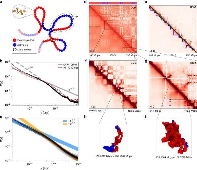
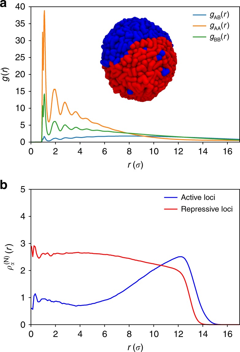
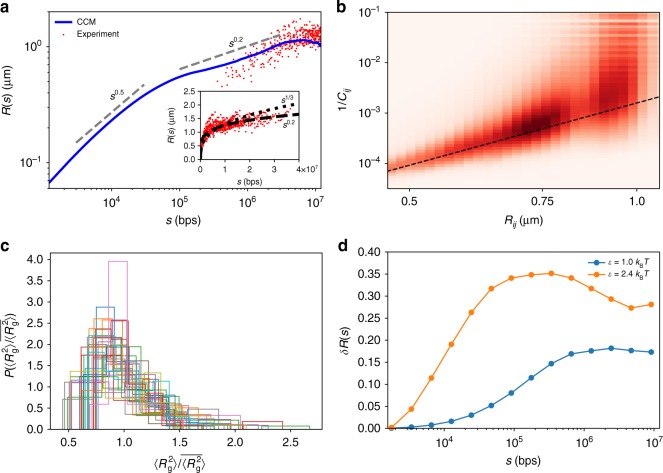
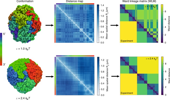
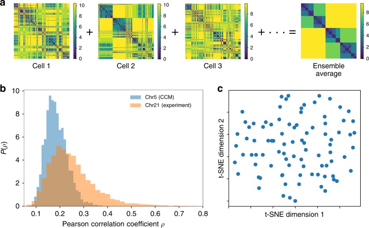
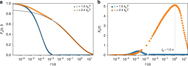
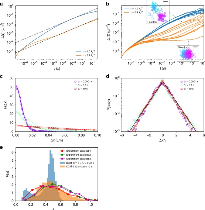
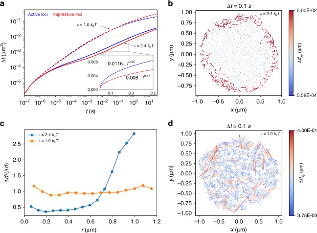
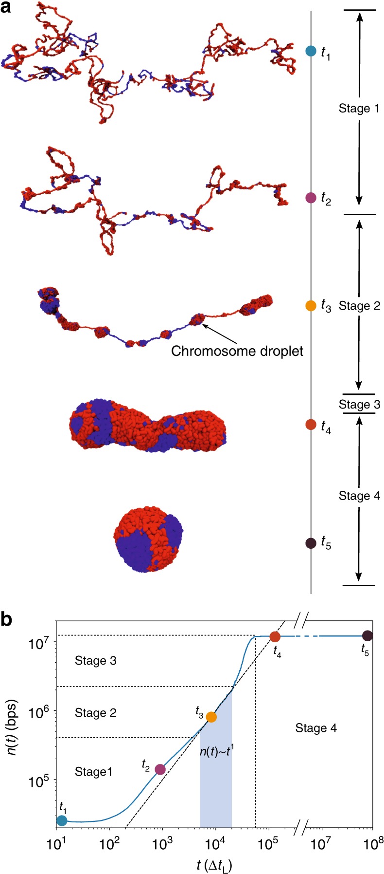
Fingerprints of the three-dimensional organization of genomes have emerged using advances in Hi-C and imaging techniques. However, genome dynamics is poorly understood. Here, we create the chromosome copolymer model (CCM) by representing chromosomes as a copolymer with two epigenetic loci types corresponding to euchromatin and heterochromatin. Using novel clustering techniques, we establish quantitatively that the simulated contact maps and topologically associating domains (TADs) for chromosomes 5 and 10 and those inferred from Hi-C experiments are in good agreement. Chromatin exhibits glassy dynamics with coherent motion on micron scale. The broad distribution of the diffusion exponents of the individual loci, which quantitatively agrees with experiments, is suggestive of highly heterogeneous dynamics. This is reflected in the cell-to-cell variations in the contact maps. Chromosome organization is hierarchical, involving the formation of chromosome droplets (CDs) on genomic scale, coinciding with the TAD size, followed by coalescence of the CDs, reminiscent of Ostwald ripening.


Conflict of interest statement

The authors declare no competing interests.

Figures

Fig. 1
Fig. 1
Comparison between the simulated contact map and the Hi-C contact map. a A sketch of the chromosome copolymer model (CCM). Each bead represents 1200 base pairs (representing roughly six nucleosomes connected by linker DNAs). Blue (red) corresponds to active (repressive) loci. The examples of three pairs of loop anchors (in this cartoon) are marked by beads with black boundaries. b Comparison between experimental data (black) and simulated P(s). Dashed and solid lines are plots of s−1.25 and s−0.75, respectively. The crossover point between the two scaling regimes at s* ~ 3 × 105 bps is noticeable in both the experimental and simulated results. c Experimental contact probability P(s) for the 23 human interphase chromosomes calculated from the Hi-C data in ref. Each black curve, all of which almost superimpose on each other, corresponds to one chromosome. Blue and orange lines are guides to the eye showing two scaling regimes. d Comparison of the contact maps inferred from Hi-C experiment (lower triangle) and obtained from simulations (upper triangle) results. For easier visualization, the values of the contact probability are converted to a log2 scale. The bar above the map marks the epigenetic states with blue (red) representing active (repressive) loci. The dashed black box is an example of a compartment. Such compartment-like structures emerge due to contacts between loci separated by large genomic distances, which gives rise to spatial order in the organized chromosome. e Illustration of topologically associated domains (TADs). The blue and green triangles are from experiments and simulations, respectively. The black circles mark the positions of loops detected from experiment data, which are formed by two CTCF motifs. f The zoom in of the diagonal region for the chromosome segment between 149.6 and 152.0 Mbps. The blue circle marks the positions of CTCF loops found in the experiment. g Same as f except for 154.4–156.8 Mbps. h, i Snapshots of two TADs, marked by the  black triangles in f and g, respectively
Fig. 2
Fig. 2
Micro-phase separation between active and repressive loci. a Radial distribution functions, g(r), as a function of r (in the unit of σ) between active–active loci (gAA(r)), repressive–repressive loci (gBB(r)) and active–repressive loci (gAB(r)). The inset shows the typical conformation of the compact chromosome. Blue and red segments correspond to active and repressive loci, respectively. The structure vividly reveals micro-phase separation between active and repressive loci. b The normalized radial density, ρα(N)(r)=Nα(r)V(4πr2ΔrNα), where Nα(r) is the number of loci of given type α found in the spherical shell between r and r + Δr, Nα is the total number of loci of that type. The bracket is the ensemble average, V is the volume of the globule, given by (43)πrmax3, where rmax = 17σ; ρα(N)(r) shows that the active loci are predominantly localized on the periphery of the condensed chromosome. The repressive loci are more uniformly distributed
Fig. 3
Fig. 3
Organization and fluctuations of the chromosome structures. a The dependence of the spatial distance R(s) (Eq.1) on the genomic distance, s. Gray dashed lines, indicating the slopes, are guides to the eye. The red dots are experimental data taken from for s < 1.2×10⁷bps. The inset shows the complete set of experimental data. Short dashed and long dashed lines are s1/3 and s0.2, respectively. At small s (s < 105bps), R(s) ~ s0.5 implying that chromatin behaves as almost an ideal chain. b The heatmap of the 2D histogram of (Rij,1/Cij). The dashed black line is the curve with scaling exponent 4.1, which coincides with the value obtained by fitting the experimental data. c Distribution P(Rg2Rg2¯), where Rg2 is the time average value of the squared radius of gyration of a single trajectory and Rg2¯ is the mean value averaged over all independent trajectories. Different colors represent P(Rg2Rg2¯) for the 32 individual TADs. The distribution is surprisingly wide, which suggests that TAD structures vary from cell-to-cell. d Coefficient of variation δR(s) = (R2(s)-R(s)2)12R(s), computed from simulations, shows a non-monotonic dependence on s for ϵ = 2.4kBT, increasing till s ~ 105 bps and decreases at larger s
Fig. 4
Fig. 4
Chromosome structure in terms of ward linkage matrix (WLM). (Left) Typical conformations of the organized chromosome for ϵ = 1.0kBT (upper) and 2.4kBT (bottom). The coloring corresponds to genomic distance from one endpoint, ranging from red to green to blue. (Middle) The ensemble averaged distance maps. (Right) Comparison between the simulated WLMs (upper triangle) and the experiment WLM (lower triangle) inferred from Hi-C contact map. Ward distance is defined in the Supplementary Note 9
Fig. 5
Fig. 5
Structural heterogeneity in the chromosome. a Ward linkage matrices of different individual cells. The single-cell WLM is the time average result over a single trajectory. The ensemble average WLM (rightmost) and the experimental WLM are in clear quantitative agreement (Fig. 4). However, the spatial organization show large variations from cell-to-cell. Each cell has very different WLM, implying their structures are distinct. b The distribution of ρ, P(ρ), with a mean ρ¯ = 0.2 (blue curve), where ρ is the Pearson correlation coefficient between WLMs of any two cells. The P(ρ) distribution, spanning the low range of ρ values, is a further demonstration of structural heterogeneity in individual cells. In yellow we plot P(ρ) with ρ¯ = 0.25 for 120 individual human interphase Chr 21, computed using the single-cell WLMs constructed from experimental measured spatial distance data provided in ref. c Two-dimensional t-SNE (t-distributed stochastic neighboring embedding) visualizations of WLM of simulated individual Chr 5 using the distance metric 1-ρ
Fig. 6
Fig. 6
Chromosomes exhibit glassy dynamics. a Intermediate scattering function obtained for ϵ = 1.0kBT (blue) and ϵ = 2.4kBT (orange). The line shows an exponential function fit, Fs(k,t), for ϵ = 1.0kBT. For ϵ = 2.4kBT, Fs(k,t)~e-(ttα)β with β = 0.27, for t exceeding a few milliseconds (black curve). b The fourth order susceptibility, χ4(t), used as a function to demonstrate dynamic heterogeneity. The peak in χ4(t) for ϵ = 2.4kBT around tM ≈ 1 s is a signature of heterogeneity
Fig. 7
Fig. 7
Dynamic heterogeneity of individual loci. (Top) a Mean square displacement, Δ(t), as a function of time, t. The effective diffusion coefficients, D, computed from the fitted dashed lines are 0.122 μm2/t0.45 and 0.009 μm2/t0.46 for ϵ = 1.0kBT and ϵ = 2.4kBT, respectively. b Time dependence of 10 single loci MSD (sMSD, Δi(t)) corresponding to 1st, 1000th,..., 10,000th loci for ϵ = 1.0kBT and ϵ = 2.4kBT. The insets show Δi(t) for two trajectories for fast (top) and slow (bottom) loci. Cyan (magenta) indicates short (long) lag times. The scale bar is 35 nm (0.07 nm) for fast (slow) loci. Caging effect can be clearly observed as the plateau in Δi(t) for ϵ = 2.4kBT. c The Van Hove function Px) for ϵ = 2.4kBT at lag times Δt = (0.0001,0.1,10)s. Px) has heavy tail at large Δx and cannot be fit by a Gaussian (color dashed lines) except for Δt = 0.0001 s at small Δx. d Same as c except displacement Δx is normalized by its standard deviation γ. Px/γ) for different lag times collapse onto a master curve. The black line is an exponential fit, ~eηx/γ) with η ≈ 1.3. e Distribution, P(α), of the effective diffusion exponent α. Comparison to experimental data are shown. The values of α are extracted from single loci trajectories by fitting sMSD, Δi(t) ~ tα. The lag time range 0.42 s < Δt < 10 s is in the approximate same range probed in the experiment. Experimental data set 1, 2, 3 are from Fig. 2b, c, and S5 of ref. , respectively. The results from our simulation (orange) agree well with experimental data, shown as orange. The blue bar plot is P(α) for small lag times 10−6 s < Δt < 0.42 s. It shows two peaks, indicating the coexistence of two populations of loci with distinct mobilities
Fig. 8
Fig. 8
Mobility of active and repressive loci. a The mean square displacement for active loci and repressive loci. The equation shown in the inset is the fit using Dtα, where D is the diffusion coefficient and α is the diffusion exponent. b The displacement vectors of the loci within the equator cross-section of the structured chromosome for ϵ = 2.4kBT. The displacements are computed for time window Δt = 0.1 s. The color bars on the right show the magnitudes of the displacements. c Displacement Δd normalized by its mean as a function of radial position, r, of the loci. d Same as b except the results are obtained using ϵ = 1.0kBT
Fig. 9
Fig. 9
Dynamics of chromosome organization. a Typical conformations sampled during the chromosome organization process. After the short initial folding process (stage 1, t1 and t2), the chromosome droplets (CDs) connected by “tension strings” begin to form (stage 2, t3). The average size of CDs at the onset of CD formation is about s ~ 4 × 105 bps, which coincides with approximate value of s*, the typical size of TADs (Fig. 1b). At the later stage (stage 3, conformation not shown here), CDs merge to form larger cluster, eventually form the final condensed structure (stage 4, t4 and t5). Red (blue) represents repressive (active) loci. b The time-dependent growth of CDs, n(t), which is the average number of base pairs in a CD at t. The dashed line is a fit in the time window indicated by the shaded area, yielding n(t) ~ t1. The roughly linear increase of n(t), over a range of times, is consistent with the Lifshitz–Slazov growth mechanism. For a vivid demonstration, see Supplementary Movie 1

Similar articles

Cited by

References

    1. Lupiáñez DG, et al. Disruptions of topological chromatin domains cause pathogenic rewiring of gene-enhancer interactions. Cell. 2015;161:1012–1025. doi: 10.1016/j.cell.2015.04.004. - DOI - PMC - PubMed
    1. Almassalha LM, et al. Macrogenomic engineering via modulation of the scaling of chromatin packing density. Nat. Biomed. Eng. 2017;1:902–913. doi: 10.1038/s41551-017-0153-2. - DOI - PMC - PubMed
    1. Dixon JR, et al. Topological domains in mammalian genomes identified by analysis of chromatin interactions. Nature. 2012;485:376–380. doi: 10.1038/nature11082. - DOI - PMC - PubMed
    1. Lieberman-Aiden E, et al. Comprehensive mapping of long-range interactions reveals folding principles of the human genome. Science. 2009;326:289–293. doi: 10.1126/science.1181369. - DOI - PMC - PubMed
    1. Rao SS, et al. A 3D map of the human genome at kilobase resolution reveals principles of chromatin looping. Cell. 2014;159:1665–1680. doi: 10.1016/j.cell.2014.11.021. - DOI - PMC - PubMed

Publication types

LinkOut - more resources