

A guide to analysis and reconstruction of serial block face scanning electron microscopy data
- PMID: 29333754
- PMCID: PMC5947172
- DOI: 10.1111/jmi.12676
A guide to analysis and reconstruction of serial block face scanning electron microscopy data
Abstract
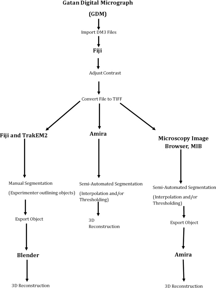
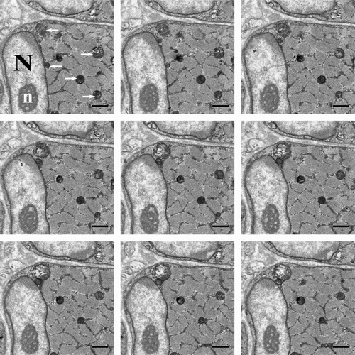
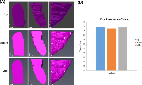
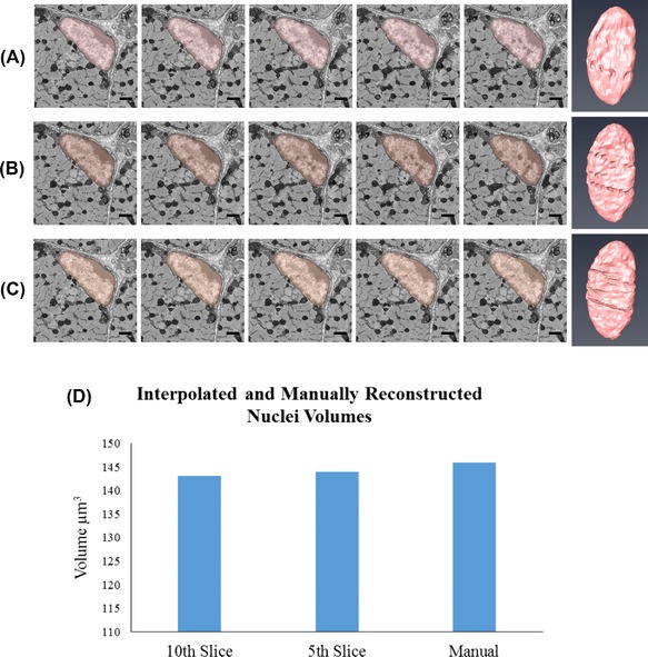
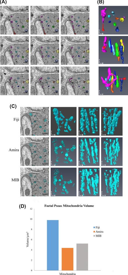
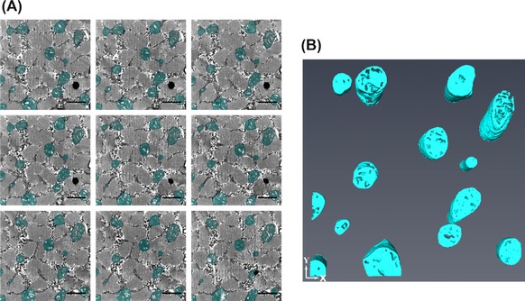
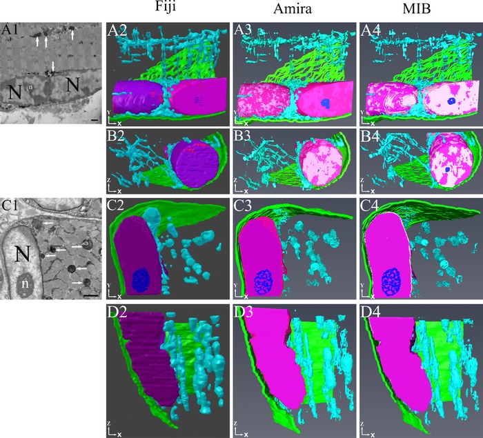
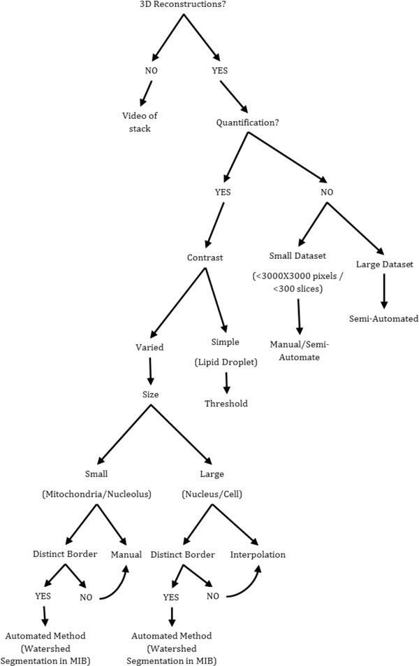
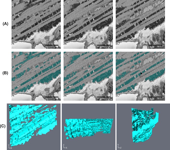
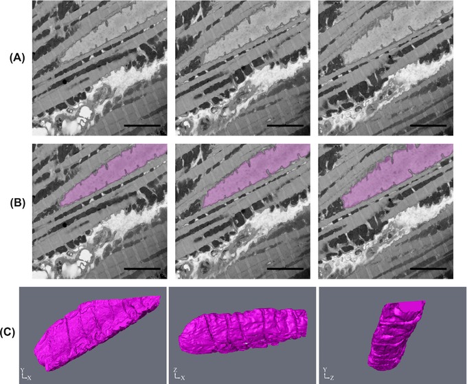
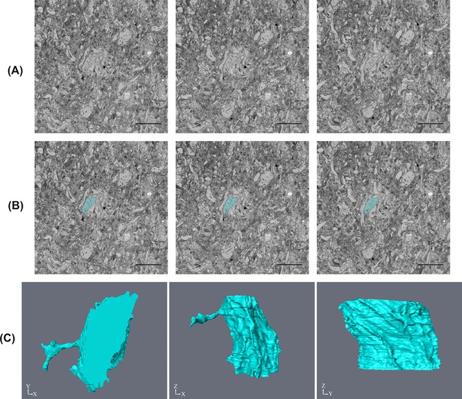
Serial block face scanning electron microscopy (SBF-SEM) is a relatively new technique that allows the acquisition of serially sectioned, imaged and digitally aligned ultrastructural data. There is a wealth of information that can be obtained from the resulting image stacks but this presents a new challenge for researchers - how to computationally analyse and make best use of the large datasets produced. One approach is to reconstruct structures and features of interest in 3D. However, the software programmes can appear overwhelming, time-consuming and not intuitive for those new to image analysis. There are a limited number of published articles that provide sufficient detail on how to do this type of reconstruction. Therefore, the aim of this paper is to provide a detailed step-by-step protocol, accompanied by tutorial videos, for several types of analysis programmes that can be used on raw SBF-SEM data, although there are more options available than can be covered here. To showcase the programmes, datasets of skeletal muscle from foetal and adult guinea pigs are initially used with procedures subsequently applied to guinea pig cardiac tissue and locust brain. The tissue is processed using the heavy metal protocol developed specifically for SBF-SEM. Trimmed resin blocks are placed into a Zeiss Sigma SEM incorporating the Gatan 3View and the resulting image stacks are analysed in three different programmes, Fiji, Amira and MIB, using a range of tools available for segmentation. The results from the image analysis comparison show that the analysis tools are often more suited to a particular type of structure. For example, larger structures, such as nuclei and cells, can be segmented using interpolation, which speeds up analysis; single contrast structures, such as the nucleolus, can be segmented using the contrast-based thresholding tools. Knowing the nature of the tissue and its specific structures (complexity, contrast, if there are distinct membranes, size) will help to determine the best method for reconstruction and thus maximize informative output from valuable tissue.
Electron microscopes have been used for decades to image cellular detail at high magnification. However the resulting images are 2‐dimensional. The development of an electron microscope in which we can section tissue in situ means that we can now acquire stacks of images giving us detail in 3‐dimensions. However the challenge with these large datasets is to reconstruct features of interest to form a 3D model. There are a number of computer programs that can be used to do this but they are not intuitive and can be overwhelming for researchers new to them. Here we explain terminology used in the programs and provide a step‐by‐step guide with accompanying videos to help researchers get started with their image analysis and get the best from their data.
Keywords: Amira; Fiji; blender; image analysis; microscopy image browser; serial block face scanning electron microscopy; skeletal muscle.
© 2018 The Authors. Journal of Microscopy published by John Wiley & Sons Ltd on behalf of Royal Microscopical Society.
Figures

Similar articles
-
A correlative approach for combining microCT, light and transmission electron microscopy in a single 3D scenario.Front Zool. 2013 Aug 3;10(1):44. doi: 10.1186/1742-9994-10-44. Front Zool. 2013. PMID: 23915384 Free PMC article.
-
A workflow for 3D-CLEM investigating liver tissue.J Microsc. 2021 Mar;281(3):231-242. doi: 10.1111/jmi.12967. Epub 2020 Oct 27. J Microsc. 2021. PMID: 33034376
-
Serial block face scanning electron microscopy for the study of cardiac muscle ultrastructure at nanoscale resolutions.J Mol Cell Cardiol. 2014 Nov;76:1-11. doi: 10.1016/j.yjmcc.2014.08.010. Epub 2014 Aug 20. J Mol Cell Cardiol. 2014. PMID: 25149127 Review.
-
Protocols for Generating Surfaces and Measuring 3D Organelle Morphology Using Amira.Cells. 2021 Dec 27;11(1):65. doi: 10.3390/cells11010065. Cells. 2021. PMID: 35011629 Free PMC article.
-
Development of protocols for the first serial block-face scanning electron microscopy (SBF SEM) studies of bone tissue.Bone. 2020 Feb;131:115107. doi: 10.1016/j.bone.2019.115107. Epub 2019 Oct 24. Bone. 2020. PMID: 31669251 Free PMC article. Review.
Cited by
-
Serial Block-Face Scanning Electron Microscopy (SBF-SEM) of Biological Tissue Samples.J Vis Exp. 2021 Mar 26;(169):10.3791/62045. doi: 10.3791/62045. J Vis Exp. 2021. PMID: 33843931 Free PMC article.
-
Serial Block Face-Scanning Electron Microscopy as a Burgeoning Technology.Adv Biol (Weinh). 2023 Aug;7(8):e2300139. doi: 10.1002/adbi.202300139. Epub 2023 May 28. Adv Biol (Weinh). 2023. PMID: 37246236 Free PMC article. Review.
-
Membrane imaging in the plant endomembrane system.Plant Physiol. 2021 Apr 2;185(3):562-576. doi: 10.1093/plphys/kiaa040. Plant Physiol. 2021. PMID: 33793889 Free PMC article.
-
Unusual nuclear structures in male meiocytes of wild-type rye as revealed by volume microscopy.Ann Bot. 2023 Dec 5;132(6):1159-1174. doi: 10.1093/aob/mcad107. Ann Bot. 2023. PMID: 37490684 Free PMC article.
-
Three-dimensional imaging and analysis of the internal structure of SAPO-34 zeolite crystals.RSC Adv. 2018 Oct 1;8(59):33631-33636. doi: 10.1039/c8ra05918g. eCollection 2018 Sep 28. RSC Adv. 2018. PMID: 35548840 Free PMC article.
References
-
- Andersson‐Cedergren, E. (1959) Ultrastructure of motor end plate and sarcoplasmic components of mouse skeletal muscle fiber as revealed by three‐dimensional reconstructions from serial sections. J. Ultrastruct. Res. 2, 5–191.
-
- Borrett, S. & Hughes, L. (2016) Reporting methods for processing and analysis of data from serial block face scanning electron microscopy. J. Microsc. 263, 3–9. - PubMed
LinkOut - more resources
Full Text Sources
Other Literature Sources
