. 2017 Mar 21;114(12):3103-3108.
doi: 10.1073/pnas.1621152114. Epub 2017 Mar 7.

Accurate model annotation of a near-atomic resolution cryo-EM map

Affiliations

Accurate model annotation of a near-atomic resolution cryo-EM map

Corey F Hryc et al. Proc Natl Acad Sci U S A. .

Abstract

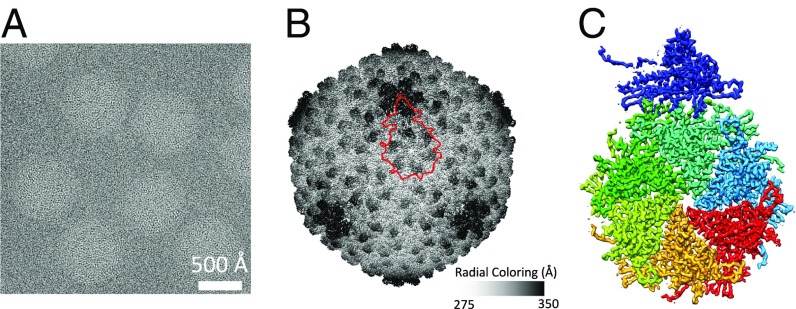
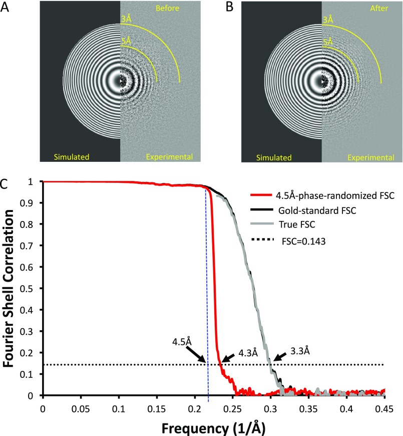
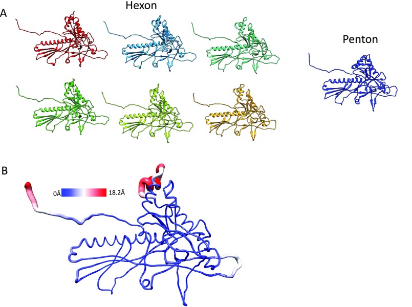
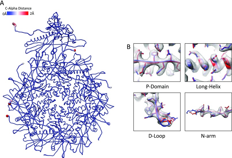
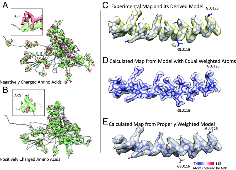
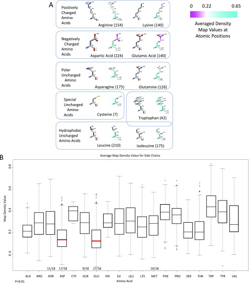
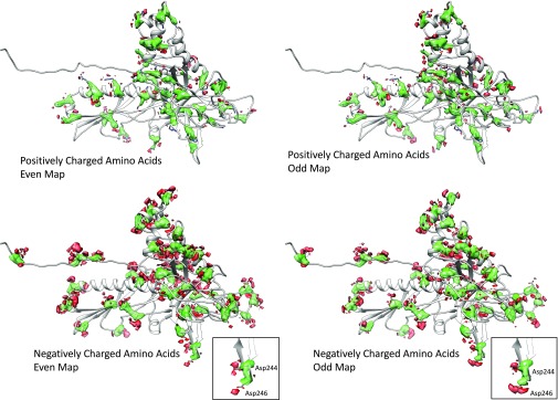
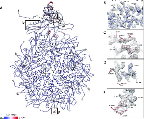
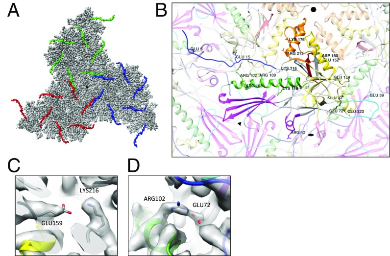
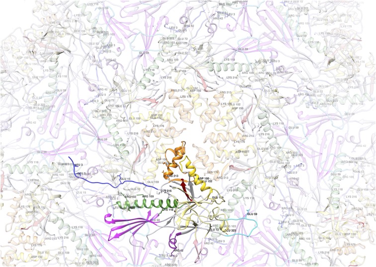
Electron cryomicroscopy (cryo-EM) has been used to determine the atomic coordinates (models) from density maps of biological assemblies. These models can be assessed by their overall fit to the experimental data and stereochemical information. However, these models do not annotate the actual density values of the atoms nor their positional uncertainty. Here, we introduce a computational procedure to derive an atomic model from a cryo-EM map with annotated metadata. The accuracy of such a model is validated by a faithful replication of the experimental cryo-EM map computed using the coordinates and associated metadata. The functional interpretation of any structural features in the model and its utilization for future studies can be made in the context of its measure of uncertainty. We applied this protocol to the 3.3-Å map of the mature P22 bacteriophage capsid, a large and complex macromolecular assembly. With this protocol, we identify and annotate previously undescribed molecular interactions between capsid subunits that are crucial to maintain stability in the absence of cementing proteins or cross-linking, as occur in other bacteriophages.

Keywords: P22; annotation; cryo-EM; model; structure.


Conflict of interest statement

The authors declare no conflict of interest.

Figures

Fig. 1.
Fig. 1.
Cryo-EM data and map. (A) Micrograph of P22 mature virion particles after motion correction and radiation damage compensation. (B) Complete 3.3-Å density map with an asymmetric unit outlined in red. (C) An asymmetric unit from the cryo-EM density map has been segmented from the complete capsid, and the seven individual capsid proteins comprising the asymmetric unit are colored differently.
Fig. S1.
Fig. S1.
(A and B) Power spectra of a typical specimen image area of the P22 bacteriophage before and after specimen motion correction and both with electron radiation damage compensation. (C) Fourier shell correlation plots computed from even and odd maps using unmodified particle images and phase-randomized particle images beyond 4.5 Å, respectively.
Fig. 2.
Fig. 2.
Cryo-EM map-derived models and model validation. (A) Domains from a hexon subunit revealing atomic-level details of the cryo-EM density map and its corresponding molecular model. (B) Overlapping the seven individual models reveals the small nuances and similarities between the capsid proteins. (C) Two FSC curves are computed for the even and odd density maps and the even model. These curves show that overfitting did not occur, as the odd map and even model are slightly worse than the even map and its corresponding model.
Fig. S2.
Fig. S2.
(A) The corresponding models, generated from the individual capsid proteins. (B) Model deviation is shown between the seven subunits. The N arm has a large variation, in addition to a small helix in the A domain, which folds inward in the penton subunit to accommodate the fivefold symmetry.
Fig. S3.
Fig. S3.
Independent models were generated for both the even and odd density maps. (A) An asymmetric unit comparing the Cα-variation between the two optimized models (even/odd model). (B) When analyzing variation at the side-chain level, it is apparent that regions with strong positive density show little amounts of uncertainty (P domain, long helix). The opposite is true for regions with weaker density, correlating with higher amounts of model variation and uncertainty (D loop and N arm).
Fig. 3.
Fig. 3.
Density map values for atomic positions for instances of the 20 amino acids. An optimized molecular model is colored by the corresponding map value. The map is rendered at a threshold of 0.22 sigma, which corresponds to white on the model. Atoms that lie in strong density are shown in cyan, whereas weak/negative density is shown in magenta.
Fig. 4.
Fig. 4.
Assessing the experimental map and corresponding model, and proper representation of the experimental data derived from the molecular model itself. (A) Density surrounding negatively charged amino acids is shown, with green representing strong positive density and red representing weak, negative density. Note the negative cloud-like density surrounding the negatively charged residues. (Inset) A specific Asp residue. (B) Density surrounding positively charged amino acids is highlighted with the same threshold as used in A. (Inset) A specific Arg residue. (C) Experimental map density and model for the spine helix are shown. (D) Currently, when creating a map from a model, all atoms are weighted equally, as shown; however, this is not a proper representation of the experimental density map. (E) The model-derived map of this helix, with proper ADPs and density weights. It faithfully recreates the experimental density map, including uncertainty/weak density in the map, and also negative map values (Fig. S7) that exist at the individual atoms themselves.
Fig. S4.
Fig. S4.
(A) Average map values, per atom, are shown for all amino acids. The numbers in parentheses represent the number of amino acids present in an asymmetric unit and averaged. For each amino acid, on the left, and colored by element, the side chains are labeled based on atom notation; for instance, CA represents the Cα-atom. The side chain on the right is colored based on its map value, and annotated with the average map value. (B) Average map value for side chains, excluding the Cα-atom. The median value is the line inside the box, the box represents the location of 50% of all observed map density values for that amino acid, the whiskers represent the maximum and minimum nonoutlier values, and the circles represent statistically proven outliers. An all-versus-all comparison of these side-chain average map values was computed. The number of statistically significant differences is shown over the number of comparisons for selected residues. It should be noted that glycine was not compared and a comparison between an amino acid and itself was not computed. Thus, 18 comparisons in total were computed per amino acid. These analyses show that the density values of ASP and GLU are significantly different from those of other residues.
Fig. S5.
Fig. S5.
Positive and negative density for even and odd maps. Density surrounding positively charged amino acids is shown on top, with green representing strong positive density and red representing weak, negative density. Density surrounding negatively charged amino acids is shown in green and the negative density in red with the same threshold on the bottom. We further draw attention to the negative cloud-like density (Insets) that surrounds the negatively charged residues. Finally, it should be noted that the half maps, displayed here, are at the closest threshold to the combined maps displayed in other figures. Small density variations do exist when comparing half density maps and combined density maps.
Fig. S6.
Fig. S6.
Atomic displacement parameters were generated per atom. (A) An asymmetric unit is shown with the average ADPs per residue mapped onto the model. (BE) Various regions in A are highlighted at the atomic level to show the variation of ADP values with respect to the map density. It should be noted that to improve visualization, the boxed regions in A are not a one-to-one spatial representation of BE.
Fig. S7.
Fig. S7.
Schematic of model-based density with two atoms having varying map values, resolution, and corresponding map values (signal). Circles represent atoms, whereas the corresponding density is represented by curves. (A) When resolution is high enough and the level of uncertainty (ADP) is low, individual map value peaks can be easily identified and two neighboring atoms will have a minimal signal between them. (B) The same is true for neighboring peaks with a positive and negative density at the atomic position. (C) If resolution is decreased or the ADP is higher, the two neighboring atoms will not have clear, delineated peaks of signal but more of a constructive interference. Combining the signal of the two positive atoms will result in the signal (Right) with two peaks and (perhaps) a shallow valley separating them. (D) Two atoms at low resolution/high ADP with opposite density would create a zero-like density (shown in the purple rectangle) when combining signal from the respective densities. Note that “negative” refers to the density of the map at the atom, not its charge, although, in fact, negative electron scattering factors are only associated with negatively charged oxygen atoms, in the case of proteins. (E and F) Properly weighted model superimposed with calculated maps revealing both positive (green) and negative (red) density computed from the model itself. Density was isolated from the (E) positively and (F) negatively charged amino acids. A comparison between the experimental and calculated map is shown in the boxes from two representative negatively charged amino acids.
Fig. S8.
Fig. S8.
Comparison of our experimental map versus maps calculated from equal weighting (PDB ID code 2MRC) and our proper weighting procedure. (A) Cross-correlation values were computed per amino acid between the experimental map and the calculated map. A 4-Å zone around the amino acid was used to isolate the density, and an average was taken across the asymmetric unit. All amino acids were better-represented using the experimental map as opposed to the equally weighted map. (B) An FSC was computed between the map and the model, using both the properly weighted map and the equally weighted map as the calculated map.
Fig. 5.
Fig. 5.
Capsid–protein interactions critical for capsid stabilization. (A) N-terminal arms from three asymmetric units stretch across to neighboring ASUs. Every one of these N-terminal arms makes an antiparallel β-strand pair with one from a neighboring subunit, even for subunits not shown. All three ASUs are tied together through potential hydrogen bonds using the N-terminal arms at the threefold axis. (B) A vast array of potential salt bridges for one subunit is highlighted. These salt bridges are commonly found between individual subunits and their neighboring subunits. (C) A representative salt bridge between Glu159 and Lys216. This salt bridge is between neighboring subunits at the base of the A domain. (D) Another salt bridge between Arg102, of the spine helix, and Glu72 in the E loop from the neighboring subunit.
Fig. S9.
Fig. S9.
Larger, more global view of Fig. 5B with additional labels highlighting the residues that are key in salt-bridge interactions.

Similar articles

Cited by

References

    1. Kühlbrandt W. Cryo-EM enters a new era. eLife. 2014;3:e03678. - PMC - PubMed
    1. Henderson R. Overview and future of single particle electron cryomicroscopy. Arch Biochem Biophys. 2015;581:19–24. - PubMed
    1. Chen S, et al. High-resolution noise substitution to measure overfitting and validate resolution in 3D structure determination by single particle electron cryomicroscopy. Ultramicroscopy. 2013;135:24–35. - PMC - PubMed
    1. Wang Z, et al. An atomic model of brome mosaic virus using direct electron detection and real-space optimization. Nat Commun. 2014;5:4808. - PMC - PubMed
    1. King J, et al. Structure and assembly of the capsid of bacteriophage P22. Philos Trans R Soc Lond B Biol Sci. 1976;276(943):37–49. - PubMed

Publication types