

Why weight? Modelling sample and observational level variability improves power in RNA-seq analyses
- PMID: 25925576
- PMCID: PMC4551905
- DOI: 10.1093/nar/gkv412
Why weight? Modelling sample and observational level variability improves power in RNA-seq analyses
Abstract
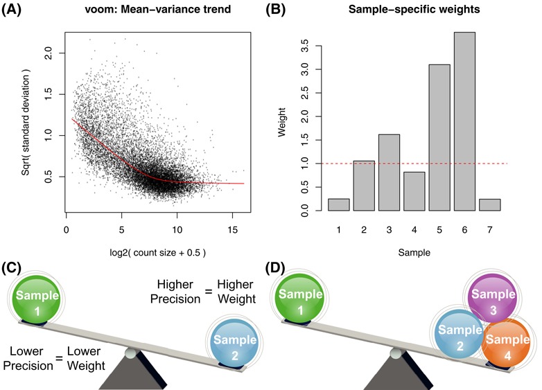
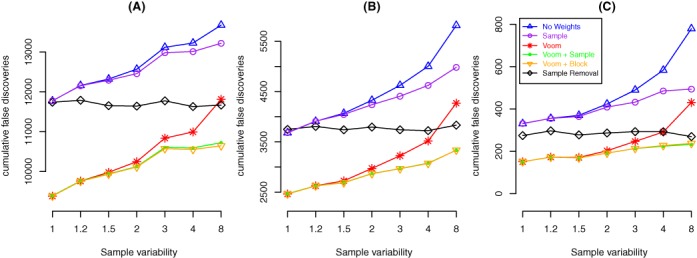
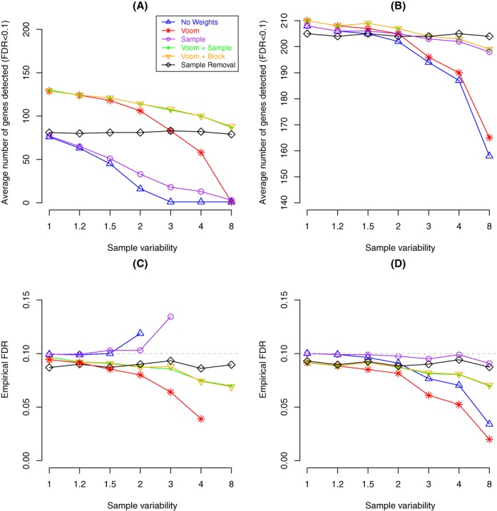
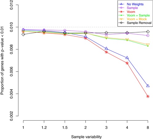
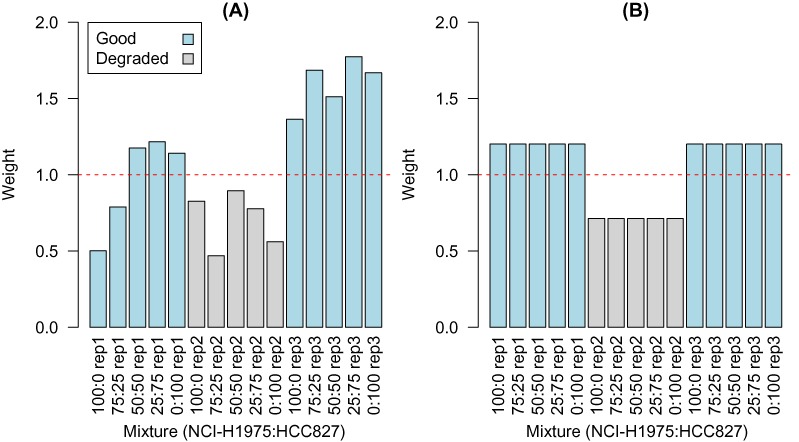
Variations in sample quality are frequently encountered in small RNA-sequencing experiments, and pose a major challenge in a differential expression analysis. Removal of high variation samples reduces noise, but at a cost of reducing power, thus limiting our ability to detect biologically meaningful changes. Similarly, retaining these samples in the analysis may not reveal any statistically significant changes due to the higher noise level. A compromise is to use all available data, but to down-weight the observations from more variable samples. We describe a statistical approach that facilitates this by modelling heterogeneity at both the sample and observational levels as part of the differential expression analysis. At the sample level this is achieved by fitting a log-linear variance model that includes common sample-specific or group-specific parameters that are shared between genes. The estimated sample variance factors are then converted to weights and combined with observational level weights obtained from the mean-variance relationship of the log-counts-per-million using 'voom'. A comprehensive analysis involving both simulations and experimental RNA-sequencing data demonstrates that this strategy leads to a universally more powerful analysis and fewer false discoveries when compared to conventional approaches. This methodology has wide application and is implemented in the open-source 'limma' package.
© The Author(s) 2015. Published by Oxford University Press on behalf of Nucleic Acids Research.
Figures

Similar articles
-
Differential expression analysis of RNA sequencing data by incorporating non-exonic mapped reads.BMC Genomics. 2015;16 Suppl 7(Suppl 7):S14. doi: 10.1186/1471-2164-16-S7-S14. Epub 2015 Jun 11. BMC Genomics. 2015. PMID: 26099631 Free PMC article.
-
No counts, no variance: allowing for loss of degrees of freedom when assessing biological variability from RNA-seq data.Stat Appl Genet Mol Biol. 2017 Apr 25;16(2):83-93. doi: 10.1515/sagmb-2017-0010. Stat Appl Genet Mol Biol. 2017. PMID: 28599403
-
It's DE-licious: A Recipe for Differential Expression Analyses of RNA-seq Experiments Using Quasi-Likelihood Methods in edgeR.Methods Mol Biol. 2016;1418:391-416. doi: 10.1007/978-1-4939-3578-9_19. Methods Mol Biol. 2016. PMID: 27008025
-
Measuring differential gene expression with RNA-seq: challenges and strategies for data analysis.Brief Funct Genomics. 2015 Mar;14(2):130-42. doi: 10.1093/bfgp/elu035. Epub 2014 Sep 18. Brief Funct Genomics. 2015. PMID: 25240000 Review.
-
The power and promise of RNA-seq in ecology and evolution.Mol Ecol. 2016 Mar;25(6):1224-41. doi: 10.1111/mec.13526. Epub 2016 Mar 1. Mol Ecol. 2016. PMID: 26756714 Review.
Cited by
-
The CALERIE™ Genomic Data Resource.bioRxiv [Preprint]. 2024 Aug 22:2024.05.17.594714. doi: 10.1101/2024.05.17.594714. bioRxiv. 2024. Update in: Nat Aging. 2024 Dec 13. doi: 10.1038/s43587-024-00775-0. PMID: 39229162 Free PMC article. Updated. Preprint.
-
Egr2 and 3 control inflammation, but maintain homeostasis, of PD-1high memory phenotype CD4 T cells.Life Sci Alliance. 2020 Jul 24;3(9):e202000766. doi: 10.26508/lsa.202000766. Print 2020 Sep. Life Sci Alliance. 2020. PMID: 32709717 Free PMC article.
-
Temporal Dynamic Methods for Bulk RNA-Seq Time Series Data.Genes (Basel). 2021 Feb 27;12(3):352. doi: 10.3390/genes12030352. Genes (Basel). 2021. PMID: 33673721 Free PMC article. Review.
-
The moss-specific transcription factor PpERF24 positively modulates immunity against fungal pathogens in Physcomitrium patens.Front Plant Sci. 2022 Sep 15;13:908682. doi: 10.3389/fpls.2022.908682. eCollection 2022. Front Plant Sci. 2022. PMID: 36186018 Free PMC article.
-
NEDDylated Cullin 3 mediates the adaptive response to topoisomerase 1 inhibitors.Sci Adv. 2022 Dec 9;8(49):eabq0648. doi: 10.1126/sciadv.abq0648. Epub 2022 Dec 9. Sci Adv. 2022. PMID: 36490343 Free PMC article.
References
Publication types
MeSH terms
Substances
LinkOut - more resources
Full Text Sources
Other Literature Sources
Molecular Biology Databases
