Review
. 2012 Sep;9(3):219-63.
doi: 10.1016/j.plrev.2012.06.001. Epub 2012 Jun 13.

Evolutionary dynamics of RNA-like replicator systems: A bioinformatic approach to the origin of life

Affiliations
Review

Evolutionary dynamics of RNA-like replicator systems: A bioinformatic approach to the origin of life

Nobuto Takeuchi et al. Phys Life Rev. 2012 Sep.

Abstract

We review computational studies on prebiotic evolution, focusing on informatic processes in RNA-like replicator systems. In particular, we consider the following processes: the maintenance of information by replicators with and without interactions, the acquisition of information by replicators having a complex genotype-phenotype map, the generation of information by replicators having a complex genotype-phenotype-interaction map, and the storage of information by replicators serving as dedicated templates. Focusing on these informatic aspects, we review studies on quasi-species, error threshold, RNA-folding genotype-phenotype map, hypercycle, multilevel selection (including spatial self-organization, classical group selection, and compartmentalization), and the origin of DNA-like replicators. In conclusion, we pose a future question for theoretical studies on the origin of life.


Figures

Figure 1
Figure 1. Survival of a non-fittest
A: The equilibrium concentrations of genotype classes (zd) are plotted against the mutation rate per digit (1 − q). The thick broken line represents the fittest genotype class (z0); the thick solid line, the second fittest genotype class (zν); the thin solid line, the third fittest genotype class (zν−1); the dotted lines, the other genotype classes. The parameters were as follows: ν = 50; AiG0 = 10; AiGν = 9.9; AiGν−1 = 2; AiGd = 1 where 0 < d < ν − 1. The results were obtained by numerically calculating the dominant eigenvector of the matrix (Bij) where Bij = AkGj Mij. The total concentration is scaled to 1 (this is always the case unless otherwise stated; see also Footnote 3). B: The equilibrium concentrations of genotypes (xi) are plotted against the mutation rate (1 − q). xi is calculated as xiGd=zd/(νd) where (νd) is the number of genotypes in a genotype class Gd. The parameters were the same as in A.
Figure 2
Figure 2. Error threshold
A: The equilibrium concentrations of genotype classes (zd) are plotted against the mutation rate (1 − q). The thick line represents the fittest genotype (z0); the thin lines, the mutant genotype classes (zd>0). The inset shows the equilibrium concentrations of genotypes (xi). In the inset, the thick line represents the fittest genotype; the thin lines, the mutant genotypes. xi was calculated as zd/(νd) where (νd) is the number of genotypes in a genotype class Gd. The parameters were as follows: ν = 50; AiG0 = 10; AiGd≠0 = 1. B: The ancestor distribution (ad) is plotted against the mutation rate (1 − q). The inset shows the ancestor distribution with respect to genotypes ad/(νd) rather than genotype classes. The parameters were the same as in A.
Figure 3
Figure 3. No error threshold
A: The equilibrium concentrations of genotype classes (zd) are plotted against the mutation rate (1 − q). The thick line represents the fittest genotype (z0), the thin lines, the mutant genotype classes (zd>0). The inset shows the equilibrium concentrations of genotypes (xi). In the inset, the thick solid line represents the fittest genotype; the dotted lines, the mutant genotypes. xi was calculated as zi/(νi). The parameters were as follows: ν = 50; AiGd = 1.05d. B: The ancestor distribution (ad) is plotted against the mutation rate (1 − q). The inset shows the average Hamming distance of the ancestor distribution from the fittest genotype 〈dad = ∑d add as a function of the mutation rate. The parameters were the same as in A.
Figure 4
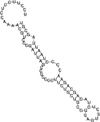
Figure 4. An example of RNA secondary structures
The RNA molecule depicted in this figure is the most abundant one at the end of the evolutionary simulation shown in Fig. 6 (time = 417650). The secondary structure was obtained with Vienna RNA Package [68]. The sequence is superimposed to the secondary structure.
Figure 5
Figure 5. Evolution in the RNA folding genotype-phenotype map
The number of generations required for the system to discover a target structure is plotted against the length of RNA sequences (the error bars show SD). One generation is defined as the total number of replication events divided by the (target) total population size (1000). The graph also shows the average Hamming distance between initial sequences and the first molecules that achieved target structures. Each data point was obtained from 100 simulation runs. For each run, two RNA sequences were randomly generated (each base with an equal chance). One sequence was used to define the target structure; the other sequence, the initial population of RNA molecules. In each time step, every molecule replicated with a probability proportional to its fitness and was removed from the system with a probability proportional to ϕ defined in a way similar to the definition of ϕ in Eq. 1 (ϕ = (1/c0) ∑i fi where fi denotes the fitness of an RNA molecule i, c0 the target population size (c0 = 1000)). The fitness of molecules was defined as 1.5d where d is the structural distance between their secondary structures and the target structure. The structural distance was defined as the number of base pairs that must be opened and closed to transform one structure into another. The mutation rate was set such that (1 − q)ν = 0.5 where ν denotes sequence length, and 1 − q a mutation rate per base.
Figure 6
Figure 6. Dynamics of RNA evolution toward a target structure
A simulation was done with the model described in Fig. 5 (ν = 76; q = 0.999). The target structure was the same as shown in Fig. 4. A: The structural distance of a current population to the target structure (population mean and population minimum). B: The mean Hamming distance between all sequences in a population (i.e. genetic heterogeneity). C: The mean Hamming distance between a current population and the initial population (gray). The Hamming distance between the fittest sequence in a current population and the initial sequence (black). D: λ is the fraction of neutral substitutions in all possible single-base substitutions in a sequence; 〈λ〉 is its population mean. MSD/time is the mean square displacement of the consensus sequence per generation [76]. The “running ave.” is the running average of MSD/time.
Figure 7
Figure 7. Dynamics of well-mixed hypercycle systems
Numerical solutions of Eq. 12 are shown for hypercycles with various numbers of members. The coordinate is the concentration xi of a hypercycle member (∑i xi is normalized to 1), and the abscissa is time. A: 3-member hypercycle. The dynamics has a stable steady state. B: 4-member hypercycle. The dynamics has an asymptotically stable steady state (the real part of the dominant eigenvalue is 0). The inset shows dynamics for longer duration. C: 5-member hypercycle. The dynamics displays oscillation. D: 9-member hypercycle. The amplitude of oscillations is greater than that in C. The parameters were as follows: kij = 1 if i = j + 1 (1 ≤ j ≤ n − 1) or if i = 1 and j = n; otherwise, kij = 0. xi(0) = 0.1 for in, and xn(0) = 1 − ∑in xi(0).
Figure 8
Figure 8. Spiral wave formation in hypercycles
The upper panels show the dynamics of hypercycles obtained with Eq. 12. Colors represent different members of a hypercycle. The parameters were the same as in Fig. 7. For n < 5 (the number of members), the initial condition was also the same as in Fig. 7. For n ≥ 5, xi(0) = 0.1 for i > 2, x1(0) = 0.11 and x2(0) = 0.11. The lower panels show snapshots of simulations with the CA model. Colors correspond to those in the upper panels. Reactions (including diffusion) were prohibited to occur across the lattice boundaries. The rate constants were the same as in Fig. 7. The diffusion rate was set to 1 (see Ref. [59]). The lattice size was 512 × 512 points (hereafter this is true unless otherwise stated).
Figure 9
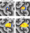
Figure 9. Core-periphery differentiation
The spatiotemporal dynamics of rotating spiral waves is depicted by consecutive snapshots of a simulation (n = 9). At t = 0, the replicators in the core of one spiral wave were colored yellow; those around the core, blue. In this blue-yellow region, one member of the hypercycle was colored red. Replicators in the other regions were colored in gray-scale. The darkest replicators and the red replicators belong to the same hypercycle member. During the simulation, every replicator “inherited” the color of the replicator from which it is replicated. The parameters were the same as in Fig. 8.
Figure 10
Figure 10. Traveling-wave formation
Snapshots depict the result of a CA model simulating the dynamics the RP system. The color coding is as follows: replicases are white; parasites, black; empty points, gray. The kP /kR ratio was chosen to be the maximum possible value for which the system can survive for a fixed value of kR (viz., kR = 0.39). The value of d is indicated in the figure. The diffusion rate was set to 0.01. The model also assumed rare mutations that transform a replicase into a parasite (10−4 per replication event). The CA was toroidal (i.e., no boundary). The lattice size was 512 × 512 points.
Figure 11
Figure 11. Generation of a new traveling wave
Consecutive snapshots depict the spatiotemporal dynamics of the CA model describing the RP system. The colors and the parameters are the same as in Fig. 10. Time goes from left to right. Only a part of the CA field is shown (75 × 75 lattice points). The second panel from left shows that replicases are left behind a propagating layer of parasites. These isolated replicases then increase their population size; concomitantly, they are infected by nearby parasites.
Figure 12
Figure 12. Evolutionary trajectories of kP and l
The lines represent the trajectories of kP and l (population averages) during evolution. The arrows indicate the values of kP and l at the beginning of simulations. The black solid line is for the model of the spatially extended RP system. The numbers beside it indicate the time points at which the snapshots of the simulation shown in Fig. 14 were taken. The dotted line and the gray line are for the model of the compartmentalized RP system and for the modification thereof, respectively (these models are described in Section 7.2.2). The parameters were as follows: kR = 0.6; κ = 1; d = 0.02. The value of kP was slightly changed (i.e., mutated) with a probability 0.01 per replication. The size of this change was uniformly distributed in the range [−0.05, 0.05]. Likewise, l was mutated as well. The two types of mutations were mutually exclusive during one replication event. In the spatially extended RP system, D = 0.1 (diffusion). In the compartmentalized RP system, D = 1 and υT = 1000 (division volume). The boundaries of the system had no flux. The lattice size was 512 × 512 points.
Figure 13
Figure 13. Life history of traveling waves
The figure shows consecutive snapshots of a simulation with the CA model with only l allowed to evolve (kP was fixed at 1). The numbers in the snapshots identify individual traveling waves. The time was reset to zero when the first snapshot was taken. The parameters were the same as in Fig. 12, except that the mutation rate of l was increased to 0.19 per replication event and that the lattice size was 1536 × 1536 points.
Figure 14
Figure 14. Evolution of traveling waves
Snapshots of the simulation taken at the three points along the evolutionary trajectory shown in Fig. 12 (black solid line).
Figure 15
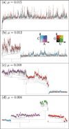
Figure 15. Phylogenetic tree of replicators
The tree was built from the genotypes (sequences) of 2000 replicators sampled from a simulation with the model explained in the main text (1 − q = 0.004). The leaves of the tree are color-coded based on the sequence composition in the dangling ends of the respective replicators. Each replicator, however, has up to four dangling ends (two ends in each of two complementary strands). Thus, one dangling end was chosen for each replicator as follows. If replicators are a replicase (i.e., if they have the catalytic structure), the 5’ dangling ends that recognize templates are chosen (i.e., the 5’ dangling end of the strands that actually fold into the catalytic structure). (Most replicases have the catalytic structure only in one strand.) The fraction of Cs and As in these dangling ends determine the colors of the corresponding leaves (the color scale is shown in the inset). If replicators are not a replicase, the 3’ dangling ends that have the most extreme sequence composition is chosen for each replicator. In this case, the colors are set to a function of the fraction of Gs and Us in these dangling ends (the color scale is shown in the inset). According to the above coloring scheme, each sequence class tends to appear as follows: C-catalysts tend to be cyan; A-catalysts, magenta; G-parasites, red; U-parasites, green. However, there are exceptions: The red leaves appearing in the clades of C-catalysts are not G-parasites, but are mutants (of C-catalysts) that have lost the catalytic structure. Thus, they belong to the C-catalyst quasi-species. Likewise, the green leaves in the clades of A-catalysts belong to the A-catalyst quasi-species. The tree was constructed with a maximum likelihood method implemented in PhyML [106]. However, owing to great divergence among sequences, the constructed tree does not necessarily depict evolutionary relationships between replicators.
Figure 16
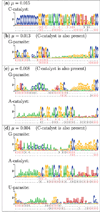
Figure 16. Typical sequence and structure of each sequence class
A sequence logo was obtained for each sequence class detected in the phylogenetic tree shown in Fig. 15. In sequence logos [107], the sizes of nucleotide characters (positively) correlate with the degree of conservation of the corresponding nucleotides in respective sequence positions. The sequence logos were generated with WebLogo [108]. The secondary structures beneath the sequence logos statistically represent the typical secondary structures in each sequence class (the structures are in the dot-bracket notation [109]). The colors of brackets indicate the frequencies of brackets in an alignment of secondary structures: the more red, the more frequent. A structure immediately beneath each sequence logo corresponds to the structure of the sequence represented by the respective logo. Below this structure is the structure of the complementary strand.
Figure 17
Figure 17. Visualization of the model system
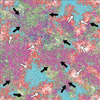
The snapshot depicts mutually invading traveling wave patterns. Each replicator is colored in the same way as the leaves of the phylogenetic tree in Fig. 15. In this coloring scheme, each sequence class appears as follows: C-catalyst (cyan); A-catalyst (magenta); G-parasite (red); U-parasite (green). The arrows represent the direction of the propagation of wave fronts: the C-catalyst fronts (black); the A-catalyst fronts (white). The CA was toroidal. The lattice size was 512 × 512 points. (A movie is also available [104].)
Figure 18
Figure 18. Evolutionary dynamics within and between compartments
Plotted is the value of kP averaged over all parasites within each compartment as a function of time. The colored squares indicate the compartments that existed in the system at the designated time. The ancestral lineages of these compartments are indicated by colored lines. The other lineages are shown by black lines. (For visibility, the values of kP are not plotted between the moments at which compartments died and those at which their last division happened.) The parameters were as follows: the value of l was fixed to 0.5; the diffusion rate was set to 1 so that a system within each compartment was relatively well-mixed; kR = 0.6; κ = 1; d = 0.02; υT = 1000 (with this value of υT the total number of replicators within a compartment was on average about 200); the lattice size, 150 × 150 points.
Figure 19
Figure 19. The death rate of compartments as a function of the stability of internal replicator systems
The death rate (i.e., the inverse of the longevity) of compartments is plotted as a function of l for various values of kP (inset, magnified view). The abscissa Δl is defined as llH. If Δl < 0, the coexistence of replicases and parasites is deterministically stable (the value of lH was obtained from an ODE model). If Δl > 0, the coexistence is deterministically unstable. The abscissa is set to Δl in order to center the curves around l = lH (lH is an increasing function of kP ).
Figure 20
Figure 20. Schematic of possible replication cycles in a replicator system with or without DNA-like replicators
RdRp denotes the RNA-dependent RNA polymerase (RNA replicase); DdRp, the DNA-dependent RNA polymerase (transcriptase); DdDp, the DNA-dependent DNA polymerase (DNA replicase); RdDp, the RNA-dependent DNA polymerase (reverse transcriptase); dual-Rp, the RNA polymerase that recognizes both RNA and DNA as templates; dual-Dp, the DNA polymerase that recognizes both RNA and DNA as templates. Superscripts indicate whether molecules are RNA or DNA.
Figure 21
Figure 21. Two-dimensional frequency histograms of Rrec and Drec
The frequencies are shown separately for the population of Rp (left panel) and the population of Dp (right panel) (populations include both RNA and DNA molecules). The gray scale is indicated in the inset. The number of bins are 20 × 20 with an equally bin size. A: the RNA-only system (Fig. 20A). The data were obtained from a simulation where the evolution of DNA molecules was disabled (i.e., with no Dp initially present in the system and μRp→Dp = 0). The parameters were as follows: κ = 1; d = 0.02; μRrec = 0.01; μDrec = 0.01; μP = 10−5; μDp→Rp = 0; υT = 500; f = 1.3 (V = fυ); the diffusion rate was 1; the boundaries had no flux, the lattice size was 512 × 512. The values of Rrec and Drec were mutated in the same manner as described in Fig. 12. B: the transcription-like system (Fig. 20C). The data were obtained from a continuation of the simulation depicted in A with the evolution of DNA molecules enabled (i.e., with μRp→Dp increased to 10−5).
Figure 22
Figure 22. Evolutionary dynamics of well-mixed replicator systems with or without DNA molecules
The model was modified such that interactions between molecules happen independently of the location of molecules (i.e., interactions are global). At the beginning of simulations, every population of RNA and DNA molecules was set in equal proportion. The initial values of Rrec and Drec were as indicated in the figure (time = 0). The parameters were the same as in Fig. 21. A: the RNA-only system (Fig. 20A). This system contains no DNA molecules; hence, Drec undergoes neutral evolution. Rrec decreases faster than Drec, that is, faster than expected for neutral evolution. B: the transcription-like system (Fig. 20C). The curves are indistinguishable from that of Drec in A, that is, from a curve expected for neutral evolution. C: the all-replicate-all system (i.e., the transcription-like system plus reverse transcription; Fig. 20D). Rrec and Drec decrease faster than Drec in A (i.e., faster than neutral evolution).

Comment in

Similar articles

Cited by

References

    1. Hogeweg P. The roots of bioinformatics in theoretical biology. PLoS Computational Biology. 2011;7:e1002021. - PMC - PubMed
    1. Phillips R, Kondev J, Theriot J. Physical Biology of the Cell. New York, NY, USA: Garland Science; 2009.
    1. Crick FHC. On protein synthesis. Symposia of the Society for Experimental Biology. 1958;12:138–163. - PubMed
    1. Crick F. Central dogma of molecular biology. Nature. 1970;227:561–563. - PubMed
    1. Moore PB, Steiz TA. The role of RNA in the synthesis of proteins. In: Gesteland RF, Cech TR, Atkins JF, editors. The RNA World. 3rd Edition. Cold Spring Harbor, NY, USA: Cold Spring Harbor Laboratory Press; 2005. pp. 257–285.

Publication types

LinkOut - more resources