. 2010 Aug 18;30(33):11232-45.
doi: 10.1523/JNEUROSCI.5177-09.2010.

Precise spatiotemporal patterns among visual cortical areas and their relation to visual stimulus processing

Affiliations

Precise spatiotemporal patterns among visual cortical areas and their relation to visual stimulus processing

Inbal Ayzenshtat et al. J Neurosci. .

Abstract

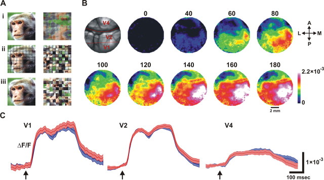
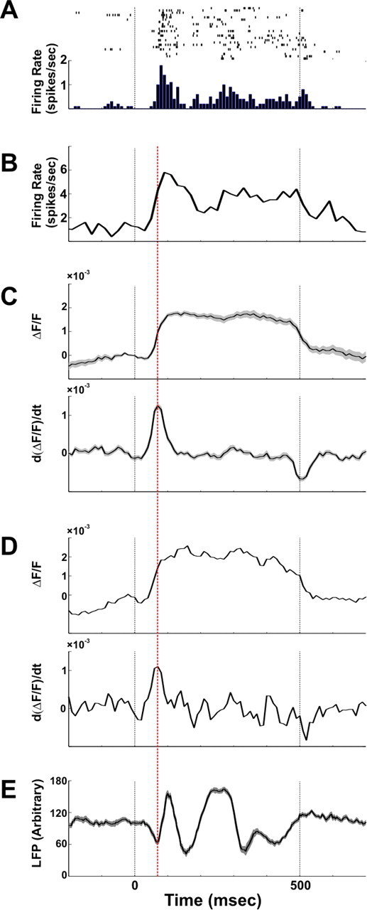
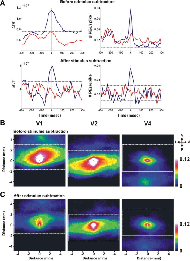
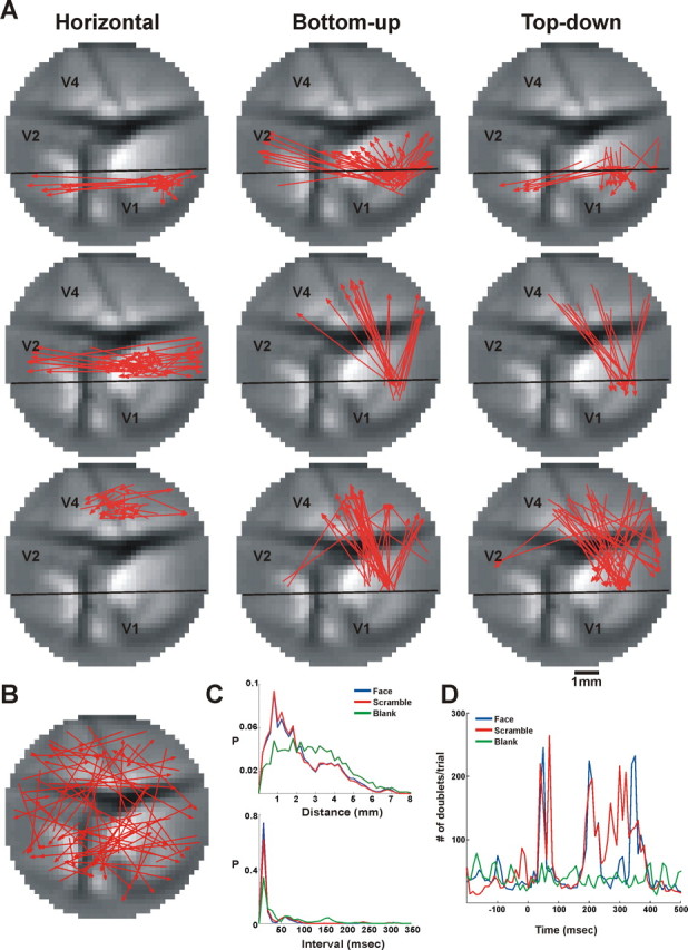
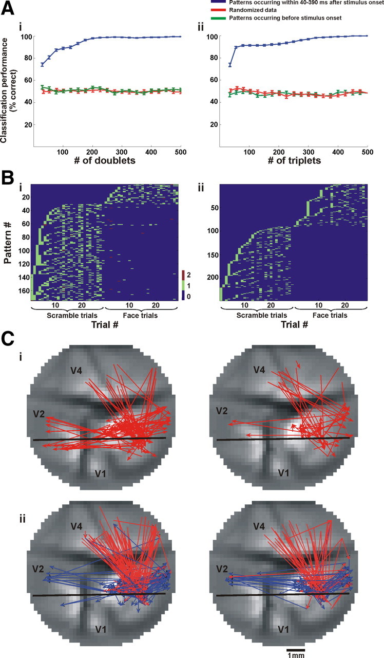
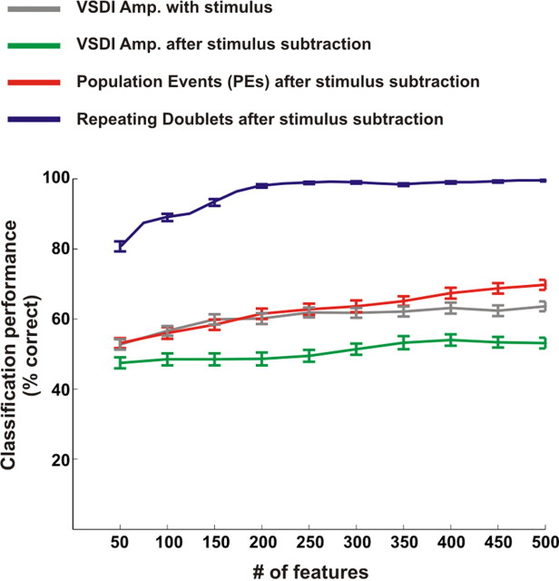
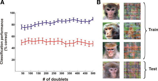
Visual processing shows a highly distributed organization in which the presentation of a visual stimulus simultaneously activates neurons in multiple columns across several cortical areas. It has been suggested that precise spatiotemporal activity patterns within and across cortical areas play a key role in higher cognitive, motor, and visual functions. In the visual system, these patterns have been proposed to take part in binding stimulus features into a coherent object, i.e., to be involved in perceptual grouping. Using voltage-sensitive dye imaging (VSDI) in behaving monkeys (Macaca fascicularis, males), we simultaneously measured neural population activity in the primary visual cortex (V1) and extrastriate cortex (V2, V4) at high spatial and temporal resolution. We detected time point population events (PEs) in the VSDI signal of each pixel and found that they reflect transient increased neural activation within local populations by establishing their relation to spiking and local field potential activity. Then, we searched for repeating space and time relations between the detected PEs. We demonstrate the following: (1) spatiotemporal patterns occurring within (horizontal) and across (vertical) early visual areas repeat significantly above chance level; (2) information carried in only a few patterns can be used to reliably discriminate between stimulus categories on a single-trial level; (3) the spatiotemporal patterns yielding high classification performance are characterized by late temporal occurrence and top-down propagation, which are consistent with cortical mechanisms involving perceptual grouping. The pattern characteristics and the robust relation between the patterns and the stimulus categories suggest that spatiotemporal activity patterns play an important role in cortical mechanisms of higher visual processing.


Figures

Figure 1.
Figure 1.
Stimuli and time course of VSDI signal. A, Example of pairs of stimuli (monkey's face and its corresponding scrambled versions). Ai shows scrambling using phase perturbations, and Aii and Aiii show segment scrambling with and without an additional grid, respectively (see Materials and Methods for details). B, Spatiotemporal activation patterns induced by the presentation of coherent face image averaged over 28 trials. Image of the blood vessel patterns (top left, red dashed lines schematically depict the borders between the cortical regions) and a sequence of frames, 20 ms apart, depict VSDI signal over the exposed visual cortex (V1, V2, and V4). Numbers represent time after the onset of the visual stimulus (milliseconds). Abbreviations: A, Anterior; P, posterior; M, medial; L, lateral. C, Time course of response. From left to right: VSDI signal amplitude in V1, V2, and V4 averaged over 427, 445, and 438 pixels, respectively. Blue trace represents the VSDI signal induced by the coherent face stimulus; red trace represents the VSDI signal induced by the scrambled face stimulus as shown in Aiii. Arrows denote the onset of the visual stimulus. Shadow area denotes SEM over 30 trials. The temporal profile averaged over pixels in V1 and V2 areas demonstrates two phases of activation; an early phase that is evoked ∼40 ms poststimulus, and a second late phase demonstrating an increase of activation ∼180 ms poststimulus.
Figure 2.
Figure 2.
Comparison of spiking activity, LFP, and VSDI signal. Example of spiking activity, LFP, and VSDI signals recorded simultaneously and evoked by a coherent face stimulus is shown. The electrophysiological recordings were performed in the same V1 area we imaged in the upper layers. A, Example of single unit activity; top shows the raster plots of 23 trials and bottom depicts the corresponding PSTH computed with 10 ms bins. B, Example of the PSTH of multiunit activity computed with 10 ms bins. C, Top shows the amplitude of the evoked VSDI signal averaged over 80 pixels located in the electrode vicinity. Bottom shows the first derivative of the VSDI signal in 20 ms sliding time window (i.e., the difference between time points 20 ms apart). D, Top and bottom show the same signals as in C only for one single pixel (located adjacent to the electrode) in one single trial. E, Mean LFP signal (21 trials, mean ± SEM). Red dashed line depicts the maximum time point in the VSDI derivative and the local minimum time point in the LFP signal. Black dashed lines depict the onset and the offset of the stimulus presentation.
Figure 3.
Figure 3.
Defining population event. Ai, Example of discretization of the VSDI analog signal from one pixel chosen in area V1. Top shows single-trial time course of the VSDI signal; middle panel shows the first derivative (blue) and threshold equal to the amplitude mean + 2SD (red); bottom panel shows the time point PEs defined as threshold crossings. Aii, Top shows example of PEs raster plots from a single trial of VSDI evoked by visual stimulus for 558, 707, and 665 pixels chosen in V1, V2, and V4, respectively. Each line in the raster represents PEs of one pixel in the imaged cortex. Bottom shows the averaged PSTH over 30 stimulus-evoked trials (note that the PSTH does not reflect small and local modulations exhibited in the raster plots above because the raster plot represents one single trial whereas the PSTH is averaged over all of the trials). Aiii, Same as in Aii for fixation-only, stimulus-free trials. Bi, Same procedure as in Ai after subtraction of the averaged VSDI signal induced by the stimulus. Left, Black trace shows the time course of VSDI signal from one pixel in area V2, green trace shows the averaged VSDI signal over 30 trials for this pixel; right, black trace shows the time course signal after subtraction of the averaged VSDI signal induced by the stimulus; bottom shows the derivative, the threshold, and the PEs for the subtracted signal. Bii, Same as in Aii, but only for trials of evoked stimulus after average VSDI signal subtraction. Red dashed line depicts the time of stimulus onset.
Figure 4.
Figure 4.
Spike-triggered average and spatial correlation maps. A, STA of the VSDI signal (averaged over 200 pixels in the electrode vicinity) in stimulus-evoked activity before and after subtraction of mean stimulus response (top and bottom, respectively). Left, Blue trace depicts the STA of the optical signal; red trace represents the shuffle condition: STA of the VSDI with spike shuffling between trials. The dashed black lines represent ±2SD from the mean of the shuffle condition (the red curve). Right, Blue trace depicts the STA of the PEs; red trace represents the shuffle condition: STA of PEs with spike shuffling between trials. The dashed black lines represent ±2SD from the mean of the shuffle condition (the red curve). Electrophysiological recordings were performed simultaneously with VSDI from upper layers. Spikes represent a multiunit activity: 418 spikes from 75 trials before stimulus subtraction and 280 spikes from 75 trials after stimulus subtraction. B, C, Averaged spatial correlation maps of PEs occurring in pixels located in areas V1, V2, and V4 (see Materials and Methods for details). The correlation maps were averaged across pixels and their PEs. The white dashed rectangles depict the size of the correlation area calculated for each pixel. The color bar depicts the correlation range measured in the matrix. Note that the central pixel, marked by an × in each map, has a correlation value of 1 by definition. We assigned this pixel a white color, indicating that the correlation value in this pixel is greater than or equal to the maximum value in the color bar. The correlation maps were calculated before removal of mean stimulus contribution (B) and after removal of the mean stimulus contribution (C). Anisotropy values before removal of mean stimulus contribution were 1.21, 2.87, and 1.41 for V1, V2, and V4 respectively, and 1.34, 2.52, and 1.47 after removal of mean stimulus contribution. Abbreviations: A, Anterior; P, posterior; M, medial; L, lateral.
Figure 5.
Figure 5.
Pattern occurrences and assessment of statistical significance. A, Example of the point processes representing all the single trials exhibiting the occurrence of one specific pattern. Ai, Trials exhibiting a pattern consisting of two PEs (doublet) from two different pixels with an interval of 10 ms. Blue and red lines denote PEs from the first and second pixel, respectively. Aii, Trials exhibiting a pattern consisting of three PEs (triplet) from three different pixels with two intervals of 10 ms each. Blue, red, and green lines denote PEs from the first, second and third pixel, respectively. Time 0 represents the onset of the visual stimulus; all the trials belong to the coherent face stimulus. B, Creating surrogate data. Illustration of PEs of four pixels and their surrogates; top illustrates PE shuffling between pixels (within a trial); bottom illustrates PE teetering within pixels. Black lines denote the original PEs; green lines denote PEs after shuffling or teetering. C, Example of the probability density function, pdf, of doublet repetition count for one imaging session and its corresponding surrogates on a log scale. Blue trace denotes the pdf of the imaging data; red, green and yellow traces denote the mean pdf of the surrogate data created by teetering the PEs within a ±10 ms time window, shuffling the PEs within cortical groups, and shuffling the PEs within illumination groups, respectively. Error bars denote ±2SD calculated over 100 generated surrogates. D, Surrogate data do not overlap with actual data. Histogram of the number of doublets repeating 30 times in surrogate data sets generated by teetering the PEs within a window of ±10 ms (we also studied teetering of up to ±5 frames, as depicted in Fig. S1, available at www.jneurosci.org as supplemental material). Two hundred surrogate data sets were independently generated. The x-axis shows the number of doublets found to repeat 30 times (using bins of size 20) in a given surrogate data set; y-axis shows the number of surrogate data sets with a given count of 30 repetition doublets. The teetering data fit a normal distribution with mean = 1035 and SD = 42.8. The actual data had a value of 1450 doublets (arrow), that is, a z-score of 9.68, which is highly significant.
Figure 6.
Figure 6.
Doublet characteristics. A, Representative doublets significantly repeating in face stimulus trials of a single imaging session. Each doublet is represented as an arrow drawn between the pixels sequentially activated in the pattern. From top to bottom: left column shows examples of horizontal doublets extending within V1, V2, and V4; middle column shows examples of bottom-up doublets (V1→V2, V1→V4, and V2→V4); right column shows examples of top-down doublets (V2→V1, V4→V1, and V4→V2). B, Representative doublets significantly repeating in blank (fixation-only) trials. The doublets shown in A and B were chosen randomly from a single imaging session, making up ∼0.2% of all the significantly repeating doublets from each group. C, The pdfs of doublet distance (top) and time intervals (bottom) that significantly repeat in trials belonging to coherent, scrambled face, and blank conditions. Both the doublet interval and the doublet distance exhibit no significant difference between the scramble and the face stimuli, and both exhibit a significant difference between the stimulus and the blank (Wilcoxon rank-sum test, p < 0.005). D, PSTH of the significantly repeating doublet occurrences; blue, red, and green traces depict face, scrambled, and blank trials, respectively. Data in AD are taken from a single imaging session, and each stimulus condition included 30 trials. Because the number of significantly repeating doublets was too large to plot them all, only a small fraction of doublets were plotted in A and B. The distributions that appear in C and the PSTH that appear in D include all the significantly repeating doublets occurring in this imaging session.
Figure 7.
Figure 7.
Readout performance of stimulus category using spatiotemporal patterns. A, Performance of binary k-nearest neighbor classifier on single-trial level as a function of the number of patterns used (blue trace, mean ± SEM, n = 50 iterations); red trace denotes performance using patterns occurring in 250 ms time window before stimulus onset (control); green trace denotes performance of the classifier trained with randomized trial category (control). Ai, Performance using doublets. Aii, Performance using triplets. Patterns were chosen according to MI rank order (see Materials and Methods for details). B, The distribution of the most informative patterns (as defined in the text) in single trials of coherent and scrambled conditions. Bi, The175 most informative doublets and their appearance in single trials. Bii, The 247 most informative triplets and their appearance in single trials. The x-axis shows the serial trial number, and the y-axis shows the pattern identification number. Note that most doublets and triplets appear uniquely either in the coherent or scrambled trials. C, The informative patterns. Ci, Doublets occurring most frequently in the scrambled-stimulus trials (left) or in the coherent-stimulus trials (right). Cii, Same as Ci for triplets. Red and blue arrows denote the first and second intervals in the triplet, respectively.
Figure 8.
Figure 8.
Comparing readout performance using various input representations. Performance of binary k-NN classifier on a single-trial level of one imaging session as a function of the number of features the classifier used. Gray and green curves show the classifier performance using single pixel VSDI amplitude before and after subtracting the average stimulus response, respectively; red curve shows the performance using PE occurrences extracted after averaged response subtraction; blue curve shows the performance using the significantly repeating doublets found after averaged response subtraction (mean ± SEM, over 50 iterations).
Figure 9.
Figure 9.
Classification of novel images. A, Performance of binary k-NN classifier trained on doublets occurring in trials of a subset of images, tested on trials of two novel images that were not included in the training set (shown in B). Each image was presented for 30 trials (blue trace, mean ± SEM, n = 50 iterations); red trace denotes performance using patterns occurring during 250 ms time window before stimulus onset (control). Data were analyzed from four recording sessions and averaged over four different combinations of train/test images. B, Example of one combination of images used for training and testing the classifier whose performance is shown in A.

Similar articles

Cited by

References

    1. Abeles M. Studies of Brain Function. Berlin: Springer; 1982a. Local cortical circuits–an electrophysiological study; pp. 62–66.
    1. Abeles M. Role of the cortical neuron: integrator or coincidence detector? Isr J Med Sci. 1982b;18:83–92. - PubMed
    1. Abeles M. Corticonics: neural circuits of the cerebral cortex. New York: Cambridge UP; 1991.
    1. Abeles M, Bergman H, Margalit E, Vaadia E. Spatiotemporal firing patterns in the frontal cortex of behaving monkeys. J Neurophysiol. 1993;70:1629–1638. - PubMed
    1. Abeles M, Hayon G, Lehmann D. Modeling compositionality by dynamic binding of synfire chains. J Comput Neurosci. 2004;17:179–201. - PubMed

Publication types

LinkOut - more resources