. 2010 Mar 12;6(3):e1000711.
doi: 10.1371/journal.pcbi.1000711.

Neocortical axon arbors trade-off material and conduction delay conservation

Affiliations

Neocortical axon arbors trade-off material and conduction delay conservation

Julian M L Budd et al. PLoS Comput Biol. .

Abstract

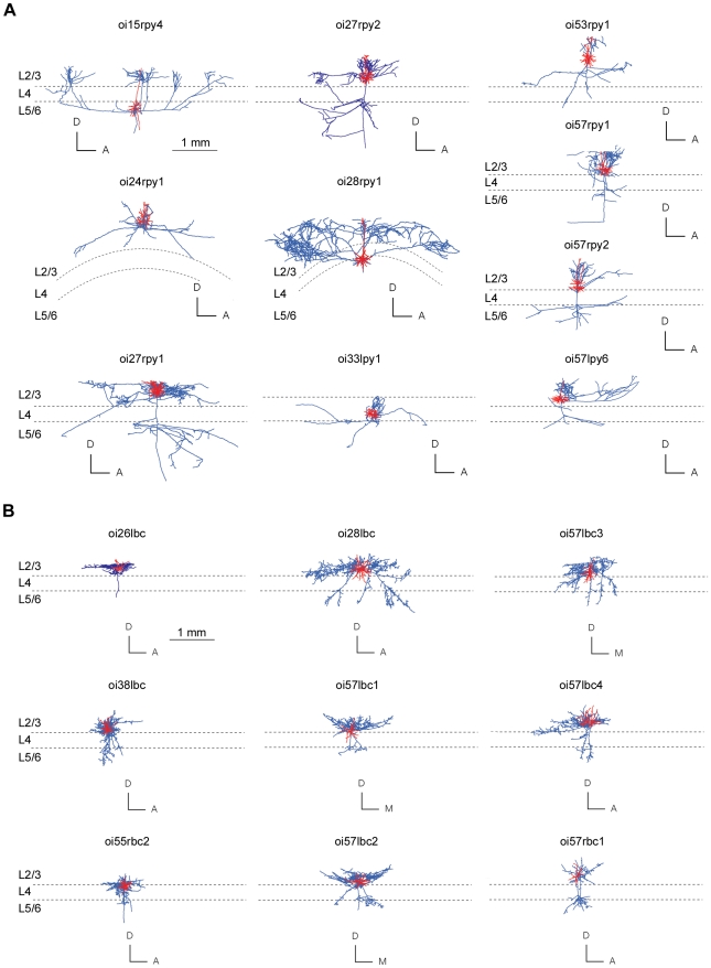
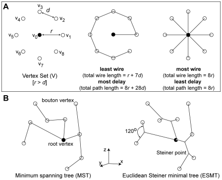
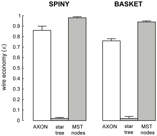
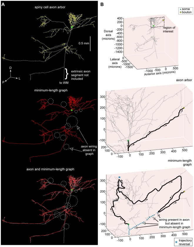
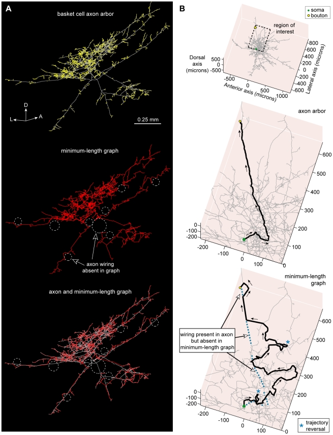
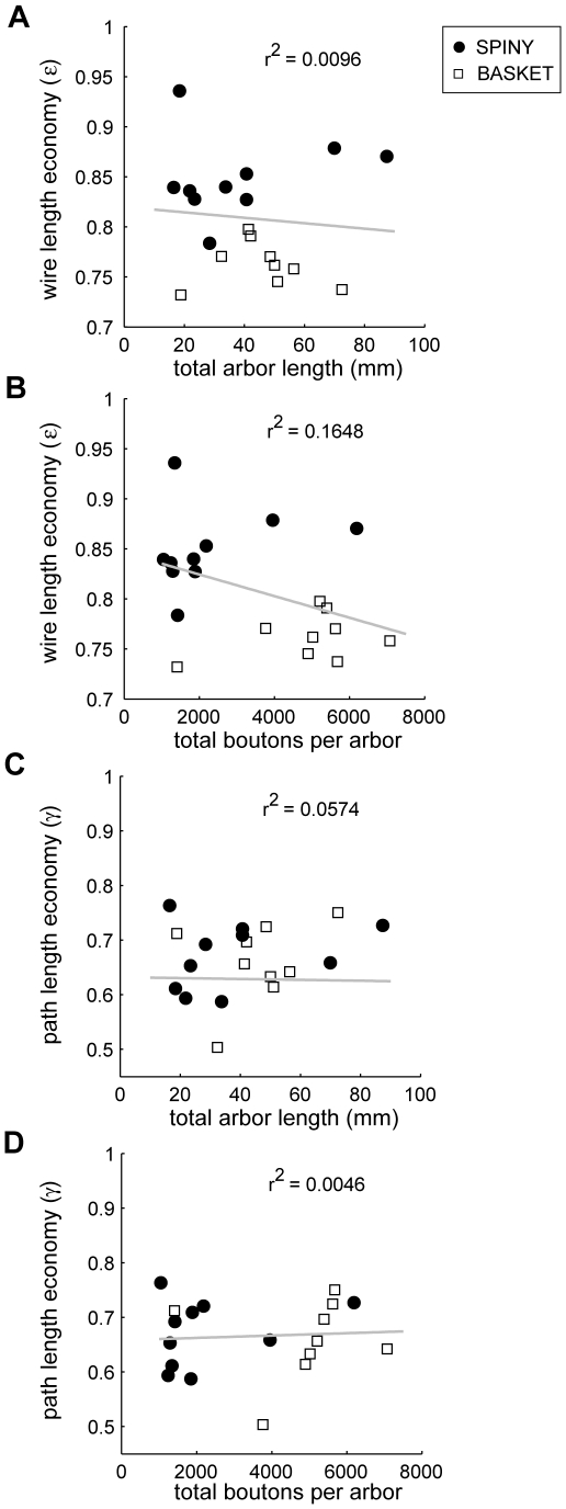
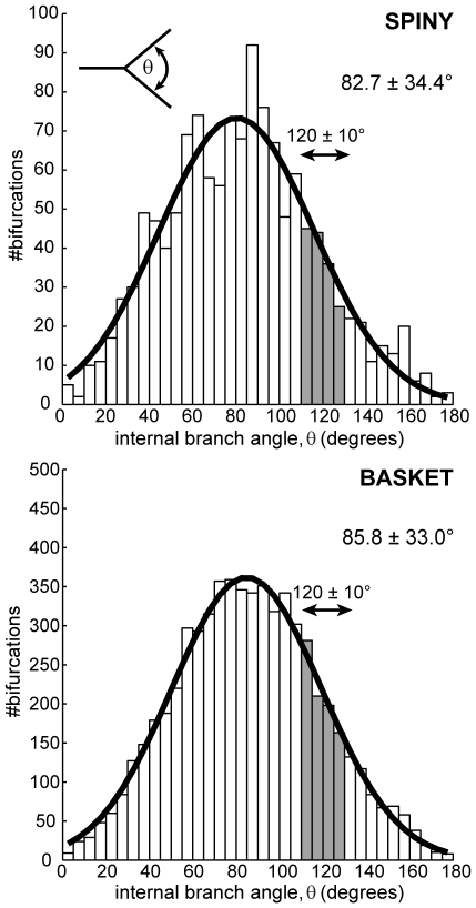
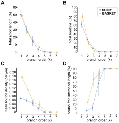
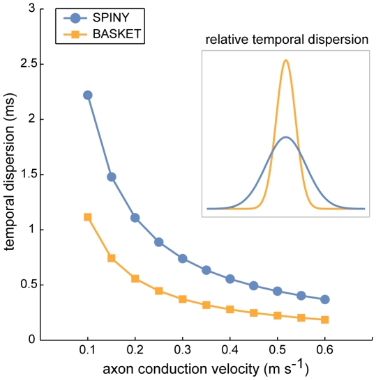
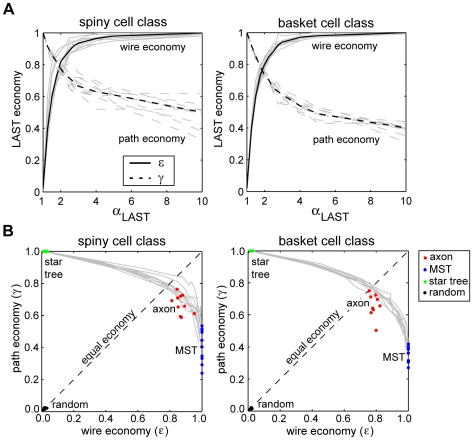
The brain contains a complex network of axons rapidly communicating information between billions of synaptically connected neurons. The morphology of individual axons, therefore, defines the course of information flow within the brain. More than a century ago, Ramón y Cajal proposed that conservation laws to save material (wire) length and limit conduction delay regulate the design of individual axon arbors in cerebral cortex. Yet the spatial and temporal communication costs of single neocortical axons remain undefined. Here, using reconstructions of in vivo labelled excitatory spiny cell and inhibitory basket cell intracortical axons combined with a variety of graph optimization algorithms, we empirically investigated Cajal's conservation laws in cerebral cortex for whole three-dimensional (3D) axon arbors, to our knowledge the first study of its kind. We found intracortical axons were significantly longer than optimal. The temporal cost of cortical axons was also suboptimal though far superior to wire-minimized arbors. We discovered that cortical axon branching appears to promote a low temporal dispersion of axonal latencies and a tight relationship between cortical distance and axonal latency. In addition, inhibitory basket cell axonal latencies may occur within a much narrower temporal window than excitatory spiny cell axons, which may help boost signal detection. Thus, to optimize neuronal network communication we find that a modest excess of axonal wire is traded-off to enhance arbor temporal economy and precision. Our results offer insight into the principles of brain organization and communication in and development of grey matter, where temporal precision is a crucial prerequisite for coincidence detection, synchronization and rapid network oscillations.


Conflict of interest statement

The authors have declared that no competing interests exist.

Figures

Figure 1
Figure 1. Morphology of spiny and basket cells analysed in study.
(A) Spiny cell axons (blue lines) and dendritic (red lines) arbors of each neuron shown in coronal plane against approximate laminar boundaries (n = 10). (B) Basket cell axons (blue lines) and dendritic (red lines) arbors of each neuron shown in coronal plane aligned with approximate laminar boundaries (n = 9). Cell identifiers matched with results given in Table S1. For clarity, axonal boutons are not shown. (Anatomical axes: A, anterior; D, dorsal; M, medial).
Figure 2
Figure 2. Artificial arbors were used to examine axonal tree optimization.
(A) Illustration of artificial arbors minimizing spatial (middle) and temporal (right) communication cost for a planar ring arrangement of bouton vertices (open circle) surrounding a cell body (filled circle) (left). For example, path p from cell body (v0) to bouton (v5) is p(v0, v5) = <v0,v1,v2,v3,v4,v5> and <v0,v5>, respectively, with corresponding path lengths dT(v0,v5) = r+4d and r. Note any given edge may be an element in more than one path but for wire length an edge is counted once only. (B) A simple 3D problem to illustrate the difference between minimum spanning tree (MST, left), where spatial cost is minimized using root and bouton vertices only, and Euclidean Steiner Minimal Tree (ESMT, right), where additional vertices called Steiner points (grey dots) may be inserted to further shorten total arbor length provided the interior angle between adjacent vertices and the Steiner point is 120°.
Figure 3
Figure 3. Wire length economy of individual spiny and basket cell intracortical axon arbors was suboptimal.
Wire length economy (ε) of spiny and basket cell intracortical axon arbors (εAXON = LMST/LAXON, where LAXON is total axon arbor length based on direct distances between boutons) compared with path length optimized star graphs (εSTAR = LMST/LSTAR) and MST with additional vertices from axon bifurcations or nodes (εMSTnodes = LMST/LMSTnodes).
Figure 4
Figure 4. Spiny cell axon arbor wiring compared with minimum-length tree.
(A) Example putative excitatory pyramidal cell axon arbor (coronal view) showing the location of numerous boutons (upper), its Euclidean Steiner Minimal Tree (ESMT) graph (middle), and overlay of axon arbor and graph (lower) with dotted circles (white) showing locations where axon wiring was absent in minimum-length graph taken to connect same bouton set. (Key: axon wiring  =  grey lines, graph wiring  =  red lines, axonal bouton  =  yellow dots, cell body  =  green dot; anatomical axes: D, dorsal; L, lateral; P, posterior.) (B) Example of the shortest path from axon origin (root vertex) of this neuron to a selected bouton (upper, see region of interest) for the biological arbor (middle) was, after branching from the main descending axon, fairly direct (0.85 mm path length) but for the length-minimized tree (lower) the route was more circuitous (2.63 mm path length), including a trajectory reversal (marked by blue asterisk), because the artificial arbor lacked wire present in the axon arbor (dotted blue lines). Arrows show direction of flow from axon origin to bouton. (Key: shortest path  =  thick black lines, unvisited arbor wiring  =  grey lines, axon wiring absent in graph  =  dotted blue lines.).
Figure 5
Figure 5. Basket cell axon arbor wiring compared with minimum-length tree.
(A) Example putative inhibitory large basket cell axon arbor (coronal view) showing bouton locations (upper), its Minimum Spanning Tree (MST) graph (middle), and overlay of axon arbor and graph (lower) demonstrating different wiring patterns used to connect same bouton set as shown by dotted circles (white). (Key: axon  =  grey lines, graph  =  red lines, boutons  =  yellow dots; anatomical axes: A, anterior; D, dorsal; L, lateral; P, posterior). (B) Example of the shortest path from axon origin (root vertex) of this neuron to a selected bouton (upper, see region of interest) for the biological arbor (middle) was initially directed away from the bouton but virtually direct thereafter (0.87 mm path length) yet for the length-minimized tree (lower) the course was tortuous (2.28 mm path length), including two trajectory reversals (see blue asterisk), because the artificial arbor lacked wire present in axon arbor (dotted blue lines). Arrows show direction of flow from axon origin to bouton. (Key: shortest path  =  thick black lines, unvisited arbor wiring  =  grey lines, axon wiring absent in graph  =  dotted blue lines.).
Figure 6
Figure 6. Wire length economy and path length economy uncorrelated with either arbor length or bouton number.
(A) Wire length economy (ε) versus total axon arbor length (LAXON) (linear regression shown as solid grey line; slope  =  −0.000272 mm−1, intercept = 0.82, r2 = 0.0096), (B) Wire length economy (ε) versus total boutons per arbor (slope  = −1.08e−5 mm−1, intercept  = 0.85, r2 = 0.1648), (C) Path length economy (γ) versus total axon arbor length (LAXON) (slope = 0.0008 mm−1, intercept  = 0.63, r2 = 0.0574), and (D) Path length economy (γ) versus total boutons per arbor (slope  = 2.16e−6 mm−1, intercept  = 0.66, r2 = 0.0046) (n = 19). The lack of correlation implies they are scale-invariant economy measures.
Figure 7
Figure 7. Axon branch points (bifurcations) are not generally Steiner points.
Distribution of local internal (aperture) angles at neocortical axon arbor bifurcations did not match Steiner point angle condition of 120° (filled bars indicate ±10° range) for either spiny (upper, 12% within ±10° range from n = 1298 nodes) or basket cell classes (lower, 14% out of n = 6192 nodes). Inset (upper) shows schematically how internal branch angle measurements were made from axon arbor reconstructions. Best-fit Gaussian distributions are shown in thick black lines (spiny, μ = 80.3°, sd = 35.7°; basket, μ = 84.8°, sd = 34.5°).
Figure 8
Figure 8. Topological ordering of an axonal tree.
(A) Strahler ordering scheme maps axonal tree topology by applying two rules to increment the order of parent branch when its descendant branches have the same order (rule 1, upper) otherwise setting the order to the maximum order of children branches (rule 2, lower). Hence, in this centripetal ordering scheme terminal branches are labelled first-order and the root branch (axon origin) given highest branch order. Example application of order scheme to whole pyramidal cell axonal tree illustrated by (B) dendrogram (right), where each vertical line was colour-coded to represent branch order (see key) and black lines represents links except for section leading to white matter (wm), with a labelled subtree (left) showing application of numbering scheme, and (C) coronal view of axon graph representation (direct distances between morphological landmarks) with colour coded branches to match the dendrogram representation shown in (B).
Figure 9
Figure 9. Axon length and number of boutons per branch order.
For both basket and spiny cell axons, with increasing branch order there was a rapid decline in (A) percentage of total axon arbor length per arbor, (B) percentage of total boutons per arbor, and (C) mean bouton density (measured from ‘bouton-laden’ axonal sections only, so ignoring ‘bouton-free’ section length from the calculation – for distinction, see text), which was initially much higher from basket than spiny cell axons. Hence, the majority of axonal wire and boutons were found on first- and second-order branches. (D) Proportion of internodal axon length per branch order accounted for by ‘bouton-free’ sections increased with branch order with an offset between spiny and basket cell classes reaching 100% at fifth-order.
Figure 10
Figure 10. Excess axonal wire originates from nature of bouton distribution, ‘bouton-free’ internodal length, and branching complexity.
(A) Whole arbor wire economy was negatively correlated with the proportion of boutons on first- and second-order branches (Spearman rank correlation, rs = −0.84, p<10−6, one-sided; linear regression (solid grey line), slope  = −109.21, intercept  = 183.35). (B) Whole arbor wire economy was strongly negatively correlated with the proportion of internodal wire length due to ‘bouton-free’ axonal sections (Spearman rank correlation, rs = −0.94, p<10−6, one-sided; linear regression, slope  = −1.93, intercept  = 1.75). (C) Average wire economy of axonal subtrees decreased with parent branch order towards whole arbor economy levels suggesting basket axon poorer wire economy was associated with their greater degree of branching complexity. (D) Percentage excess wire grew with branch order towards whole arbor levels implying each level of branching costs excess wire length in neocortical axons.
Figure 11
Figure 11. Examples of wiring ‘shortcuts’ by wire-minimization algorithms.
(A) Low economy spiny axon arbor (left upper) wiring was significantly shortened by MST (left lower) shortcuts linking bouton-rich terminal patches while avoiding bouton-free primary and secondary axon collaterals. Magnified central region (right) shows numerous wiring differences in the flow direction from soma to tips between overlaid axon (grey arrows) and MST (red arrows) arbors. (B) High economy spiny cell axon arbor (left upper) wiring was only slightly shortened because MST (left lower) could find fewer shortcuts because of the more uniform bouton distribution over the sparsely branched axon arbor. Magnified central region axon and MST overlay (right) illustrates few differences in wiring pattern flow between these arbors. (C) Cell type-specific differences in wiring shortcuts: for a typical basket cell axons wiring shortcuts zig-zag between boutons ‘strings’ on terminal branches but avoid the main bouton-free axon collateral (upper), while for a typical spiny cell branch boutons are found on all orders of branching permitting very few shortcuts (lower). (Key: axon  =  grey lines, graph  =  red lines, boutons  =  yellow dots; anatomical axes: A, anterior; D, dorsal; L, lateral; M, medial; P, posterior).
Figure 12
Figure 12. Path length economy of neocortical axons was suboptimal though superior to wire-minimized arbors.
(A) Coronal view of example spiny cell axon arbor (left) and its MST (right): upper, shows wire length minimization generally increased path length from parent cell body along arbor to each bouton (dot colour codes for path length, see scale bar), and, lower, histograms show this results in a shift in path length distribution of these arbors from positively skewed to one more dispersed and symmetric. (Anatomical axes: A, anterior; D, dorsal; L, lateral; M, medial; P, posterior). (B) Surface view of example basket cell axon arbor (left) and its MST (right) shows, upper, a similar increase in path length (note different colour scale to (A)) compared with spiny axon arbor with wire minimization, and, lower, a spread in path length distribution. (C) Path length economy (γ) of spiny (left) and basket cells axons (right) was suboptimal (γAXON = PSTAR/PAXON, where PAXON is average path length from parent soma to each bouton in the arbor) though significantly greater than wire-minimization arbors regardless of whether or not (γMST = PSTAR/PMST) these inserted additional vertices (branch points) according to Steiner minimal tree criteria (γESMT = PSTAR/PESMT) or the actual axon bifurcations or nodes (γMSTnodes = PSTAR/PMSTnodes) were used.
Figure 13
Figure 13. Neocortical axons, unlike wire-minimized arbors, preserve cortical distance-path length relationship.
(A) Spiny cell axons (top) regression line (solid green line) diverged little from optimal slope (path length/distance ratio  = 1, dotted gold line) and was much better correlated compared with MSTs either without (middle) or with axon bifurcations (nodes) as additional vertices (bottom). Black dots represent single bouton measurements, n = 22,344 boutons. (B) Basket cell axons (top) regression line likewise diverged little from optimal slope and was marginally better correlated compared with MSTs either without (middle) or with the addition of axon bifurcations (bottom), n = 44,064 boutons. (C) Spiny cell axon path length ratio distribution (black line) showed a sharp initial peak followed by a slower exponential-like decay with 82% of ratio <2 (grey shaded region), compared with the broader distributions of MSTs without (red line) and with the addition of axon bifurcations (blue line) with 33–34% only of ratio <2. (D) Basket cell axon path length ratio distribution had a similar shape to spiny cells', 78% of paths with ratio <2, while the wider distributions of MSTs without and with axon bifurcations as additional vertices, with around 12–13% of ratio <2, peaked near ratio of 3. The strong similarity between spiny and basket axon path length ratio distributions implies a common (temporal) cost constraint mechanism.
Figure 14
Figure 14. Temporal dispersion of neocortical axonal latencies was much less than wire-minimized arbors.
(A) Degree of temporal dispersion (standard deviation) of spiny cell axons latencies (left, black line), independent of conduction velocity, was six to eight times and basket cell latencies (right, black line) around three times less than corresponding MST with (blue line) or without additional axon bifurcation points (red line), suggesting wire minimization increased temporal dispersion. Addition of axon bifurcations in MSTs reduced the degree of temporal dispersion. Standard deviation was measured by deviation from the respective regression lines shown for path length in Figure 13AB. Comparison of predicted latency distributions of axon arbors and MSTs at (B) 0.15 m s−1, and (C) 0.30 m s−1 conduction velocities illustrates the sharpness of axonal temporal dispersion compared with broader wire minimization results (N.B. total number of paths constant across conditions).
Figure 15
Figure 15. Temporal dispersion of basket cell axon latencies was approximately half that of spiny cell axons.
Inset shows normalised Gaussian profiles of relative temporal dispersion independent of conduction velocity.
Figure 16
Figure 16. Neocortical axon arbor design represents a trade-off between spatial and temporal communication costs.
(A) Light-approximate spanning tree (LAST) algorithm shows for each arbor that as the maximum path length ratio determined by αLAST increased so wire and path economy proved opposing objective functions for both spiny (left) and basket cell class axon arbors (right). At around αLAST = 1.9 the separate economy curves achieve equilibrium with parameters matched at ≈0.79. Light grey curves represent individual arbor results while thick black lines represent mean economy results (solid lines  =  wire economy, dashed lines  =  path economy). (B) Relative to trade-off curves in the economy plane generated by LAST algorithm (solid grey lines) the results show spiny (left) and basket cell axons (right) were suboptimal for wire length economy (ε) compared with wire-minimized MST and were suboptimal for path length economy (γ) compared with path-minimized star trees. Most neocortical arbors lay on or near the trade-off curves with a slight bias towards wire minimization relative to equal economy line (dotted black line). In comparison, randomized trees were close to the origin of the economy plane indicating the degree of axon economy.

Similar articles

Cited by

References

    1. Laughlin SB, Sejnowski TJ. Communication in neuronal networks. Science. 2003;301:1870–1874. - PMC - PubMed
    1. Foh E, Haug H, König M, Rast A. Quantitative bestimmung zum feineren aufbau der sehrinde der katze, zugleich ein methodischer beitrag zur messung des neuropils. Microsc Acta. 1973;75:148–168. - PubMed
    1. Braitenberg V, Schüz A. Berlin, Germany: Springer-Verlag; 1991. Anatomy of the Cortex: Statistics and Geometry.
    1. Peters A, Payne BR. Numerical relationships between geniculocortical afferents and pyramidal cell modules in cat primary visual cortex. Cereb Cortex. 1993;3:69–78. - PubMed
    1. Budd JML. Extrastriate feedback to primary visual cortex in primates: a quantitative analysis of connectivity. Proc Roy Soc Lond Series B. 1998;265:1037–1044. - PMC - PubMed

Publication types

LinkOut - more resources