Review
doi: 10.1021/cr030440j.
Modeling kinetics of subcellular disposition of chemicals
Affiliations
- PMID: 19265398
- PMCID: PMC2682929
- DOI: 10.1021/cr030440j
Item in Clipboard
Review
Modeling kinetics of subcellular disposition of chemicals
Chem Rev.
2009 May.
No abstract available
Figures
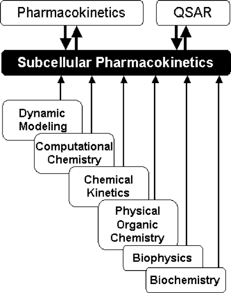
Structure-based subcellular pharmacokinetics and related sciences. Two-sided arrows indicate mutual influence; one-sided arrows indicate supportive roles.
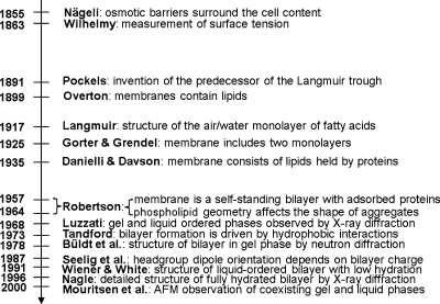
Historical milestones in the elucidation of bilayer structure.
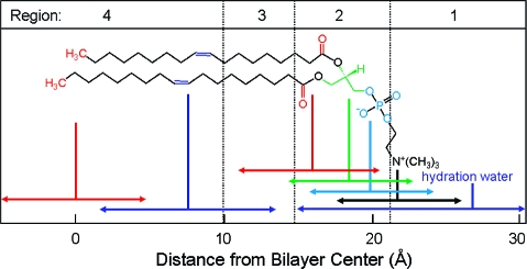
Thermal motion and subregions of the liquid-ordered dioleoylphosphatidylcholine bilayer. The arrows indicate the range of 95% probability of occurrence of (from left) terminal methyls (red), double bonds (blue), carbonyls (red), glycerol (green), phosphate (light blue), choline (black), and hydration water (blue).(220) The subregions are approximated according to the MD simulation results.(292)
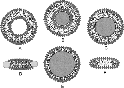
Cross sections of spherical or discoid phospholipid aggregates: (A) liposomes, (B) supported bilayers on microspheres, (C) monolayers on alkylated microspheres, (D) nanodisks, (E) immobilized artificial membranes, and (F) bicelles. The schematic structures are not drawn to proportion. More details are given in the text.
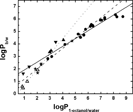
Dimyristoylphosphatidylcholine bilayer/water, versus 1-octanol/water partition coefficients(544)P for (●) nonpolar compounds, (▲) phenols, (△) alcohols, (▼) anilines, and (★) polar compounds with no hydrogen-bond donor group. Lines represent linear fits to the data for (—) nonpolar compounds, (- - -) phenols and alcohols, and (· · ·) polar compounds without hydrogen-bond donor ability. More details are given in the text.
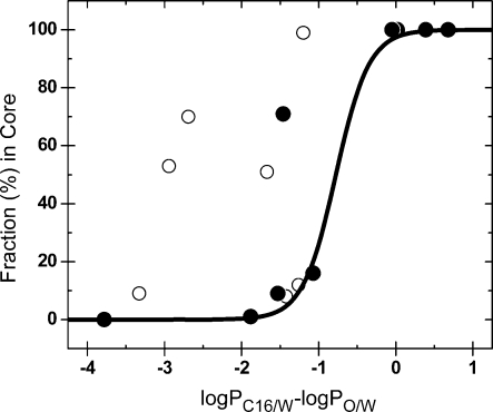
Fractions of the chemicals in the core region, as predicted from the C16/DAcPC partitioning, versus the difference between C16/W and C16/O partition coefficients. The compounds with experimentally determined locale are shown as full points. The sigmoidal curve connects the compounds with known locales in the headgroups or the core and corresponds to eq 2.(552)
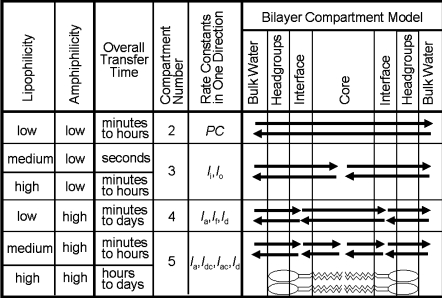
Compartmentalization of the bilayer for the description of passive transport of chemicals as dependent on lipophilicity and amphiphilicity of chemicals. The headgroups and the core are represented by the low-density bilayer subregions 1 and 4, respectively. The core/headgroups interface is depicted as a volume, where amphiphilic chemicals accumulate and includes (portions of) the high-density subregions 2 and 3. The headgroups/water interface is not shown, because of insufficient information about the accumulation of chemicals there. The schematic phospholipid structures in the bottom right corner indicate these correspondences. The overall transfer time is the time needed for a complete equilibration of a chemical across a liquid-ordered bilayer, based on the experimental data referenced in the text. The transfer rate parameters are listed in the order of individual steps, from the donor aqueous phase (left) to the acceptor aqueous phase (right). For the backward processes, the order of individual steps is in the right-to-left direction.
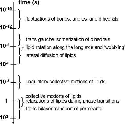
Time scales of the movements of phospholipids and permeants in a fluid phospholipid bilayer. More details are given in the text.
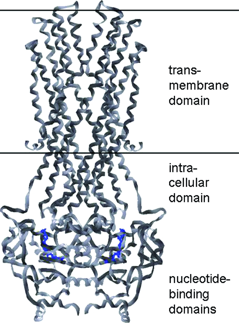
Structure of the bacterial ABC transporter Sav1866, (PDB(1173) file 2ONJ) is shown in the ribbon mode (gray). The bound molecules of the ATP analog adenosine-5′-(β,γ-imido)triphosphate are shown in blue.(1291) The approximate position of the bilayer is indicated by horizontal lines.
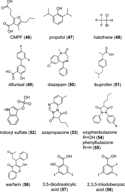
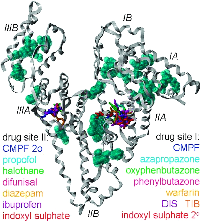
The X-ray structure of human serum albumin (HSA) with ligands bound in the drug sites I (right) and II (left). Structures of the ligands (tubes shown in colors) are summarized in Chart 4 (number, the Protein Databank (PDB) file): 3-carboxy-4-methyl-5-propyl-2-furanopropionic acid, CMPF (46, 2BXA);(1290) propofol (47, 1E7A); halothane (48, 1E7B);(1287) diflunisal (49, 2BXE); diazepam (50, 2BXF); ibuprofen (51, 2BXG); indoxyl sulfate (52, 2BXH); azapropazone (53, 2BX8); oxyphenbutazone (54, 2BXB); phenylbutazone (55, 2BXC); warfarin (56, 2BXD); 3,5-diiodosalicylic acid, DIS (57, 2BXL);(1290) and 2,3,5-trioiodobenzoic acid, TIB (58, 1BKE).(1285) The PDB(1173) files were superimposed with respect to C-α carbon atoms. The cyan spheres(1290) represent potential binding cavities identified using the Sybyl module SiteID.(1291) Many of the cavities serve as binding sites for fatty acids and thyroxine and as secondary sites for some of the shown drugs. Individual domains are marked.
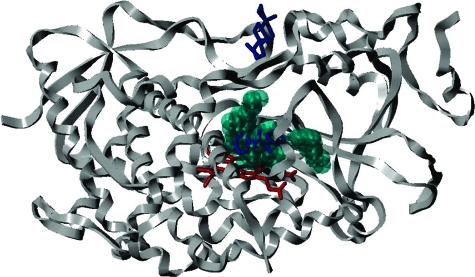
X-ray structure of human CYP3A4, with bound metyrapone (blue) shown close to the heme (red) and progesterone (blue) at the top of the protein., The PDB(1173) files 1W0F and 1W0G were superimposed with respect to C-α carbon atoms.(1291) The cyan spheres(1290) represent the binding cavity identified using the Sybyl module SiteID.(1291)
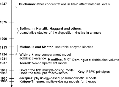
Milestones in the history of classical pharmacokinetics. More details and references are given in the text.
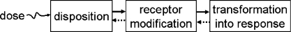
Phases of drug action. Under certain conditions (details in the text), the phases can be described by separate models, with little feedback from the subsequent process, as indicated by the dotted backward-facing arrows. Structure-based subcellular pharmacokinetics explicitly addresses disposition; however, the results are used to formulate the descriptions for the other two phases.
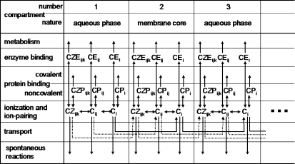
Schematic outline of the distribution of the chemicals, which do not interact with the headgroups, in a morphologically compartmentalized system consisting of alternating aqueous phases and membranes (represented by the cores). The chemicals can be present as free non-ionized molecules (Ci), free molecules ionized to the jth degree (Cij), or ion pairs with the kth counterion (CZijk); each species can be bound to proteins (P) or enzymes (E), and eliminated by spontaneous and/or enzymatic reactions. The subscripts i, j, and k are typically used throughout the paper, in the meanings that are shown here. Two-sided arrows represent fast processes, whereas one-sided arrows represent time-dependent processes.
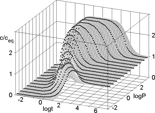
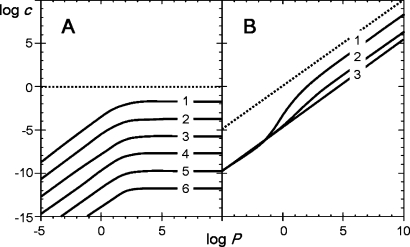
Transport kinetics in the third, aqueous compartment of a 10-compartment system (c is the concentration, the subscript “eq” denotes equilibrium, t is time), relative to lipophilicity.(2089) For compartment numbering, see Figure 14. The chemicals accumulate above the equilibrium level (c/ceq = 1) for a significant fraction of the distribution period. The data were obtained by numerical simulation of the pure transport of the compounds, which do not interact with the headgroups, in a system of alternating aqueous phases (5) and bilayers (5), with the transfer rate parameters li and lo related to the partition coefficient P according to eqs 3.(2089) The surface corresponds to eq 10 with the values of the coefficients specified in Table 5.
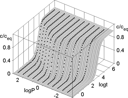
Transport kinetics in the sixth, core compartment of a 10-compartment system, relative to lipophilicty.(2089) The system consists of alternating aqueous (5) and core (5) phases. The concentrations of chemicals do not exceed the equilibrium concentrations at any moment. The surface corresponds to eq 10 with the values of the coefficients specified in Table 5. Other details are as given in Figure 15.
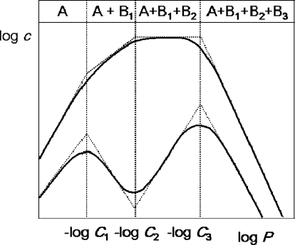
Meanings of the adjustable coefficients in eq 11 that describes the relationship between the subcellular concentrations c and lipophilicity expressed as the partition coefficients P. The slopes of the linear parts, relative to the coefficients A and Bi, are given in the upper part (all expressions are to be multiplied by the coefficient β). The positions of the curvatures are determined by the values of the coefficients Ci.(2089)
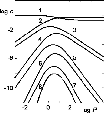
Nonequilibrium concentration−lipophilicity profiles for individual phases of a 10-compartment system of alternating aqueous and core phases at a constant time of distribution.(2089) Other details as in Figure 15. The compartment numbers are shown near the respective curves. The aqueous phases are denoted by the odd numbers and the bilayers are marked by even numbers, as in Figure 14 in section .
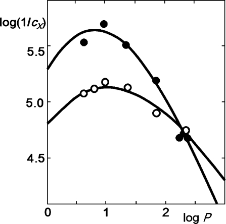
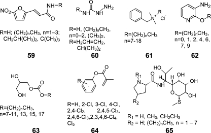
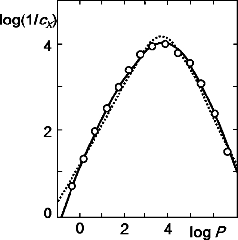
Mutagenicity of alkyl amides of 3-(5-nitro-2-furyl)-acrylic acid (59 in Chart 5) against Salmonella typhimurium TA100 rfa+ (full points) and rfa− (open points), as dependent on the 1-octanol/water partition coefficient P. The concentration cX (mol/l) elicits, under given conditions, 600 revertants per plate. The curves correspond to eq 11 with i = 1 and the optimized values of the coefficients given in the first two lines of Table 7.(2091)
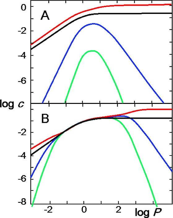
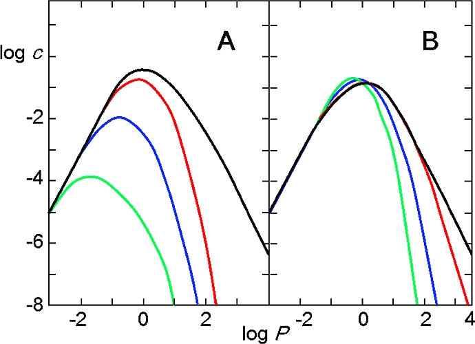
Concentration−lipophilicity profiles in the membranes of a 10-compartment system of alternating water and bilayer phases in the (A) nonequilibrium (10 time units) and (B) mixed (1000 time units) periods of distribution.(2089) Curves for compartments 2 (the first bilayer, red lines), 6 (the third bilayer, blue lines), and 10 (the fifth bilayer, green lines) are shown, along with the equilibrium curve (black lines). In compartment 2, chemicals accumulate above the equilibrium concentration in both nonequilibrium and mixed periods. The numbering is as given in Figure 14 in section , whereas other details are as shown in Figure 15 in section .
Growth inhibition of Ctenomyces mentagrophytes by alkyl amines (cX is the minimum inhibitory concentration)(2093), relative to the lipophilicity, expressed as the partition coefficient P. The dotted curve corresponds to the bilinear equation 9, and the full curve represents eq 11 for the mixed period of distribution (i = 2). The optimized coefficient values are given in Tables 8 and 9, respectively.
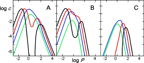
Concentration−lipophilicity profiles of chemicals in the last compartment of the water−bilayer−water−bilayer system (A) without elimination, (B) with elimination from either both aqueous phases, or (C) with elimination from the intracellular aqueous phase after the following distribution periods (in time units): 0.1 (green), 1 (blue), 100 (red), and ∞ (black).(2089) The elimination rate constants are identical for all compounds and set to zero, except k1 = k3 = 1/(time unit) in panel B and k3 = 1/(time unit) in panel C. Other details are as given in Figure 15 in section .
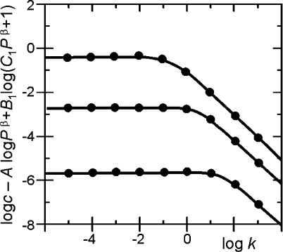
Reactivity dependence of the concentrations in compartment 4 of a four-compartment, water−bilayer−water−bilayer model that were corrected for the contribution of lipophilicity to show only the reactivity portion of this form of the disposition function (eq 13). The exposure time is increasing from top to bottom. Other details are as given in Figure 22.
Influence of protein binding on the concentration−lipophilicity profiles of nonionizable chemicals in the nonequilibrium period in the fifth aqueous compartment of a system of alternating aqueous phases and bilayers, as calculated using eq 14. Protein binding is lipophilicity-dependent, according to eq 4 with bi00 = BiPβ, Bi = B1 = B3 = B5, and B2 = B4 = 0 (see eqs 38 and 43). The transfer rate parameters li and lo are dependent on the partition coefficient P, according to eq 3. Panel A illustrates the effect of the increasing protein concentration: β = 1 and Bi = 0 (black), 0.01 (red), 1 (blue), and 100 (green). Panel B illustrates the effect of the increase in the sensitivity of binding to lipophilicity: Bi = 0 (black); and Bi = 1 and β = 0.75 (red), 1.00 (blue), and 1.25 (green).(2110)
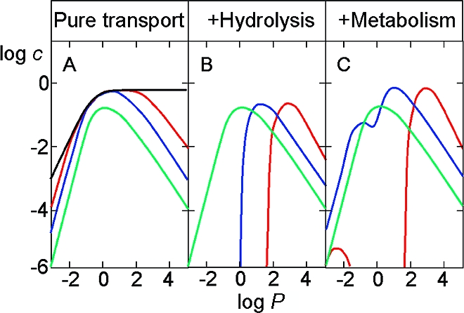
Dependencies(2112) of the concentration c in the fifth compartment of the system of alternating aqueous and bilayer phases on the partition coefficient P for (A) pure unidirectional transport, (B) transport combined with protein binding, and (C) transport influenced by protein binding and metabolism, after the following times of distribution (in time units): 3.2 (green), 10 (blue), 32 (red), and 100 (black). Calculated using eq 14, with the parameters as in Figure 24A (Bi = 1) and ki = 1/(time unit).
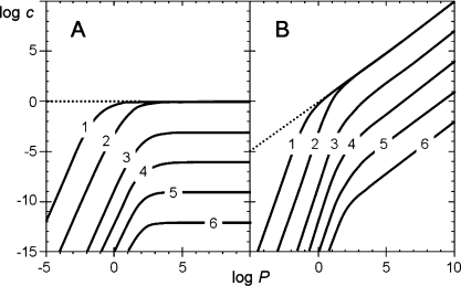
Steady-state concentrations versus lipophilicity in (A) individual aqueous phases and (B) individual bilayers for the invariant elimination rate constants. The aqueous phases are represented by compartments 3−23 and membranes are represented by compartments 2−22, both with step 4 (curves 1−6, respectively; compartment numbering is as shown in Figure 14 in section ). The curves correspond to eqs 17 and 18 with c1 = 1 unit and EM = 1 (time unit)−1. The flux terms in eqs 17 and 18 are defined in eqs 46 and only contain the surface areas and the transfer rate parameters. The transfer rate parameters are expressed by eqs 3.(2115) The dotted line indicates c1 in A and c1P in B.
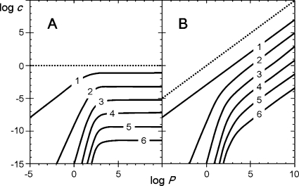
Steady-state concentration−lipophilicity profiles for (A) aqueous compartment 7 and (B) bilayer 8 of a catenary system of alternating aqueous and bilayer phases, relative to the elimination rate constant k.(2115) The elimination terms only contain k, in (time unit)−1: 10−4 (curve 1), 10−2 (curve 2), 1 (curve 3), 10 (curve 4), 102 (curve 5), and 103 (curve 6). Other details are as shown in Figure 26.
Average steady-state concentration−lipophilicity profiles in (A) all aqueous phases and (B) all bilayers of a system of alternating aqueous and bilayer phases, as a function of the elimination rate constant. Curves correspond to eqs 19 and 20, with other details as given in Figure 26. The elimination rates constants k, in (time unit)−1, are 10−4 (curve 1 in both parts), 10−2 (curve 2), 1 (curve 3), 102 (curves 4 and 3 in parts A and B, respectively), 104 (curves 5 and 3 in parts A and B, respectively), and 106 (curves 6 and 3 in parts A and B, respectively).(2115)
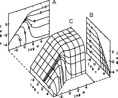
Relationship(2124) between the concentration c of the protein-bound chemical, the partition coefficient P, and the exposure time of distribution t for a pseudo-equilibrium situation: (A) projection into the plane c−P, (B) projection into the plane c−t, and (C) overall view. The values were calculated using eq 25 multiplied by P, with c0 = 1 unit, β = A = 1, B = 0.1, C = 0.01, and D = 0. Individual curves in projection A are valid for log t = −4 (curve 1), −3 (curve 2), −1.75 (curve 3), −0.5 (curve 4), 0.75 (curve 5), 1.25 (curve 6), 1.75 (curve 7), 2.75 (curve 8), 3.75 (curve 9), and 4.75 (curve 10). Individual curves in projection B are valid for log P = −4 (curve 10), −3 (curve 9), −2 (curve 8), −1 (curve 7), 0 (curve 6), 1.25 (curve 5), 2.5 (curve 4), 3.75 (curve 3), 5 (curve 2), and 6 (curve 1).(2124)
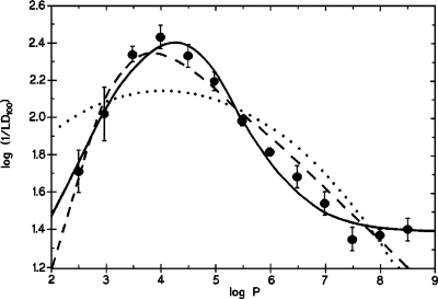
Inhibitory activity of n-alkanes in mice (LD100 in mol/kg)(64) versus lipophilicity, expressed as the 1-octanol/water partition coefficient P. Data were fitted with eq 26 (D = 0, the values of other adjustable coefficients are given in the bottom line in Table 10) (solid line),(2124) the bilinear equation described by eq 9 (dashed line), and the parabolic equation described by eq 8 (dotted line).(2124)
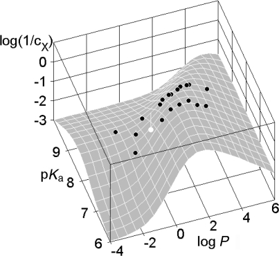
Growth-inhibiting activity of lincomycin derivatives(2190) against Sarcina lutea in the agar diffusion test, as a function of acidity, given as the negative logarithm of the dissociation constant Ka, and lipophilicity, parametrized by the 1-octanol/water partition coefficient P.(34) The surface corresponds(20) to eq 29. The fitted activities of the trans derivatives (not shown) form a similar surface, raised by 0.283 logarithmic units. The outlier did not conform to the smooth surface. More details are given in the text.
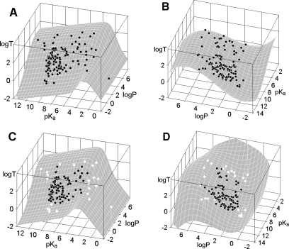
Acidity−lipophilicity−toxicity profiles for phenols against Tetrahymena pyriformis(55) generated by the model-based eq 30 (panels A and C) and the best empirical model (panels B and D) for the complete set of compounds (panels A and B) and for the reduced set of compounds (panels C and D) as used in leave-extremes-out cross validation. The omitted points in the reduced set are indicated by empty circles.(55) The model-based equations are able to predict beyond the used parameter space, whereas the empirical models fail in this aspect. Toxicity (T) values are the inverse values of the isoeffective concentrations (in mmol/L) causing 50% growth inhibition after 96 h of exposure. More details are given in the text.
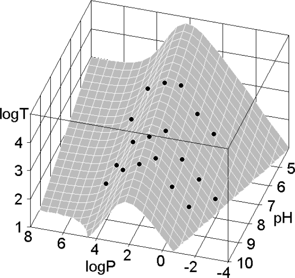
Dependence of the inhibitory activity of α-bromoalkanoic acids against V. cholerae on the 1-octanol/water partition coefficient P and the pH values of the medium. Toxicities (T) are given as the inverse values of the minimum killing concentrations. The surface corresponds to eq 34, with the optimized values of adjustable coefficients given in Table 11.(2224)
Similar articles
-
Domain formation in the plasma membrane: roles of nonequilibrium lipid transport and membrane proteins.Phys Rev Lett. 2008 May 2;100(17):178102. doi: 10.1103/PhysRevLett.100.178102. Epub 2008 Apr 28. Phys Rev Lett. 2008. PMID: 18518341
-
The 'double lives' of membrane lipids. Workshop: Anno 2000. A lipid milestone.EMBO Rep. 2001 Feb;2(2):91-5. doi: 10.1093/embo-reports/kve029. EMBO Rep. 2001. PMID: 11258718 Free PMC article. No abstract available.
-
Cooperative dynamics of quasi-1D lipid structures and lateral transport in biological membranes.Gen Physiol Biophys. 1997 Dec;16(4):311-9. Gen Physiol Biophys. 1997. PMID: 9595300
-
Thermodynamics of lipid interactions in complex bilayers.Biochim Biophys Acta. 2009 Jan;1788(1):72-85. doi: 10.1016/j.bbamem.2008.08.007. Epub 2008 Aug 15. Biochim Biophys Acta. 2009. PMID: 18775410 Review.
-
Capacities of membrane lipids to accumulate neutral organic chemicals.Environ Sci Technol. 2011 Jul 15;45(14):5912-21. doi: 10.1021/es200855w. Epub 2011 Jun 28. Environ Sci Technol. 2011. PMID: 21671592 Review.
Cited by
-
Convergence of Free Energy Profile of Coumarin in Lipid Bilayer.J Chem Theory Comput. 2012 Apr 10;8(4):1200-1211. doi: 10.1021/ct2009208. Epub 2012 Feb 24. J Chem Theory Comput. 2012. PMID: 22545027 Free PMC article.
-
Structural determinants of drug partitioning in n-hexadecane/water system.J Chem Inf Model. 2013 Jun 24;53(6):1424-35. doi: 10.1021/ci400112k. Epub 2013 May 21. J Chem Inf Model. 2013. PMID: 23641957 Free PMC article.
-
Bioanalysis of eukaryotic organelles.Chem Rev. 2013 Apr 10;113(4):2733-811. doi: 10.1021/cr300354g. Chem Rev. 2013. PMID: 23570618 Free PMC article. Review. No abstract available.
-
Structure-based prediction of drug distribution across the headgroup and core strata of a phospholipid bilayer using surrogate phases.Mol Pharm. 2014 Oct 6;11(10):3577-95. doi: 10.1021/mp5003366. Epub 2014 Sep 18. Mol Pharm. 2014. PMID: 25179490 Free PMC article.
-
A Permeability Study of O2 and the Trace Amine p-Tyramine through Model Phosphatidylcholine Bilayers.PLoS One. 2015 Jun 18;10(6):e0122468. doi: 10.1371/journal.pone.0122468. eCollection 2015. PLoS One. 2015. PMID: 26086933 Free PMC article.
References
-
- Bio-Loom Database and Software; Biobyte Corp.: Claremont, CA, 2006. (www.biobyte.com)
-
- Kurup A. J. Comput. Aid. Mol. Des. 2003, 17, 187. - PubMed
-
- Hansch C.; Steward A. R.; Iwasa J.; Deutsch E. W. Mol. Pharmacol. 1965, 1, 205. - PubMed
-
- Hansch C. Farmaco 1968, 23, 293. - PubMed
-
- Hansch C.; Dunn W. J. J. Pharm. Sci. 1972, 61, 1. - PubMed
Publication types
MeSH terms
Substances
Grants and funding
LinkOut - more resources
Full Text Sources