. 2009 Sep;15(9):1093-108.
doi: 10.1007/s00894-009-0454-9. Epub 2009 Feb 21.

Solvent accessible surface area approximations for rapid and accurate protein structure prediction

Affiliations

Solvent accessible surface area approximations for rapid and accurate protein structure prediction

Elizabeth Durham et al. J Mol Model. 2009 Sep.

Abstract

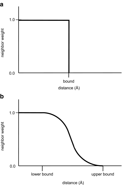
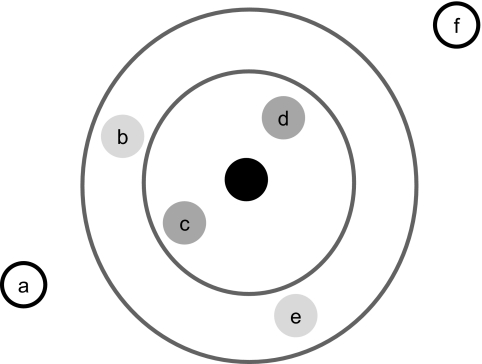
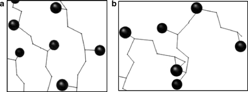
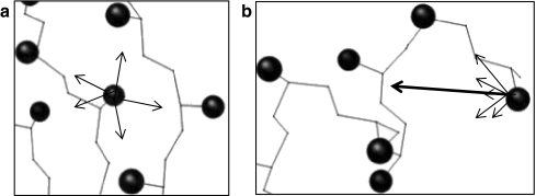
The burial of hydrophobic amino acids in the protein core is a driving force in protein folding. The extent to which an amino acid interacts with the solvent and the protein core is naturally proportional to the surface area exposed to these environments. However, an accurate calculation of the solvent-accessible surface area (SASA), a geometric measure of this exposure, is numerically demanding as it is not pair-wise decomposable. Furthermore, it depends on a full-atom representation of the molecule. This manuscript introduces a series of four SASA approximations of increasing computational complexity and accuracy as well as knowledge-based environment free energy potentials based on these SASA approximations. Their ability to distinguish correctly from incorrectly folded protein models is assessed to balance speed and accuracy for protein structure prediction. We find the newly developed "Neighbor Vector" algorithm provides the most optimal balance of accurate yet rapid exposure measures.


Figures

Fig. 1
Fig. 1
This figure depicts ways in which a “neighboring” amino acid can be defined. a) Previous work uses a step function with a hard boundary to determine which amino acids are neighbors. Any amino acids lying within that boundary are considered neighbors and any amino acids lying outside of that boundary are not considered neighbors. b) An expanded definition of neighbor that includes a smooth transition function is used in the neighbor count algorithm. Rather than a single boundary, a lower and upper boundary are designated. Amino acids lying within the lower boundary are considered complete neighbors and are assigned a neighbor weight of 1.0. Amino acids lying outside of the upper boundary are not considered neighbors at all and are assigned a neighbor weight of 0.0. Amino acids lying between the lower and upper bounds are assigned a weight between 0.0 and 1.0 based on their proximity to the amino acid of interest
Fig. 2
Fig. 2
This figure depicts the neighbor count algorithm. The inner and outer gray rings represent the lower and upper bounds respectively. The small circles represent the formula image atoms of amino acids. The black circle represents the amino acid of interest. Amino acids a and f are assigned a neighbor weight of 0.0 because they are outside of the upper bound. Amino acids b and e are assigned a weight between 0.0 and 1.0 because they lie between the upper and lower bounds. Amino acids c and d are counted as one complete neighbor each because they lie within the lower bound
Fig. 3
Fig. 3
This figure depicts a shortcoming of the neighbor count algorithm. Lines are drawn from the amino acid of interest in this case to all neighboring (as defined by the neighbor count algorithm) amino acids. Two scenarios are shown for which the neighbor count algorithm returns a value of five. However, these two scenarios depict two very different exposure states
Fig. 4
Fig. 4
This figure depicts the neighbor vector algorithm. The vectors drawn to the formula image of neighboring amino acids are shown in black and the vector sum is shown in heavyweight black. a) When summed, the vectors essentially cancel out yielding a vector of zero length which indicates burial. b) When summed, the vectors yield a vector with a large magnitude which indicates exposure
Fig. 5
Fig. 5
A β-strand is shown where the formula image atoms and formula image atoms of the strand are represented by black and white circles respectively. The formula image of neighboring amino acids are represented by white circles. The neighbor vectors are shown as dashed lines. The formula image vectors are shown as solid lines. The dot product of the neighbor vector and the formula image vector gives information about the angle between the two vectors and hence the orientation of the side chain atoms with respect to the neighboring amino acids (large open circles)
Fig. 6
Fig. 6
The overlapping spheres algorithm places a sphere around each formula image and places points on the surface of the spheres. The points that do not overlap with the spheres of any other amino acids are used as a measure of relative exposure. The formula image atoms are colored in black and the points that do not overlap with any other spheres are colored in gray. a) the exterior of the protein b) a cut away of the protein
Fig. 7
Fig. 7
The knowledge-based potentials based upon each exposure algorithm are shown and colored by value where white represents low values and dark gray represents high values. A visual inspection of the KBPs confirms that the energies shown in the KBPs agree with expectations. For example, one expects a hydrophobic amino acid, for example valine (V), to prefer a low exposure value, a large number of neighbors, and a low neighbor vector magnitude. This is in fact what is seen as indicated by the minima in the plots. Conversely, one expects a hydrophilic amino acid, such as lysine (K) to prefer a high exposure value, a small number of neighbors and a high neighbor vector magnitude. This is also what is seen in the plots
Fig. 8
Fig. 8
The average enrichment, z-score, and area under the ROC curve (AUC) is shown for each exposure algorithm over all benchmark proteins. The z-scores are in light gray, the AUC values are in medium gray, and the enrichment values are in dark gray. The neighbor count algorithm performs the least favorably according to all of the evaluation measures whereas the remaining algorithms perform approximately the same with the ANN generally performing slightly better than the others
Fig. 9
Fig. 9
The enrichment is shown for each algorithm over all benchmark proteins. There are some proteins for which none of the exposure algorithms provided an enrichment (for example 1scj) while there are some benchmark proteins for which many of the exposure algorithms provided good enrichments. There are also proteins for which the enrichment produced by each algorithm increased with algorithm complexity as expected (for example 1enh)
Fig. 10
Fig. 10
The area under the ROC curve (AUC) is shown for each exposure algorithm over all benchmark proteins. The AUC varies widely over the benchmark proteins. There are some proteins for which all algorithms perform very well (for example, 1c9o) while there are some proteins for which none of the algorithms perform well (for example, 1scj)
Fig. 11
Fig. 11
a) The ROC curve for 1enh. As the algorithm complexity increases, the area under the ROC curve increases. In this case, the OLS algorithm is able to distinguish between native-like and nonnative-like models more effectively than the reference standard rSASA algorithm. b) rSASA, enrichment: 5. c) neighbor count, 1.46. d) neighbor vector, 3.13. e) ann, 4.58. f) ols, 6.67. In b) – f) the energy scores assigned to each protein model (each protein model is represented by one point) is plotted against the rmsd100 value of that model. Models assigned an energy score in the lowest 10% (most energetically favorable) are shown as solid circles whereas models assigned an energy score in the highest 90% (least energetically favorable) are shown as open circles. If the energy potential is able to perfectly distinguish between native-like (<5 Å rmsd100) and nonnative-like (≥5 Å rmsd100) models, the 10% of models identified as most energetically favorable (shown in black) would have an rmsd100 value <5 Å. As the algorithm complexity increases, the potential based on the algorithm is able to more effectively distinguish between native-like and nonnative-like models as also indicated by the increasing enrichment values. Interestingly, the OLS algorithm achieves a higher enrichment value than the true rSASA value indicating that additional factors must be taken into account in order to capture all aspects of environment free energy
Fig. 12
Fig. 12
The backbone and formula image are shown in gray. The ALA5 formula image is shown in black. The actual relative rSASA as determined by the reference standard method of ALA5 is 0.375 and it is the 13th most exposed exposed amino acid in the protein model. Lines are drawn from the ALA5 formula image to all formula image assigned a neighbor weight >0 as determined by the neighbor count algorithm. Although ALA5 has many neighbors, all of the neighbors are on one face of the amino acid leaving the other face exposed. Therefore, the neighbor count algorithm ranks ALA5 only as the 21st most exposed amino acid. The neighbor vector algorithm is able to distinguish that most of the neighboring amino acids are on one face of ALA5 and ranks ALA5 as the 19th most exposed amino acid in the protein model. The ANN is able to use the NC, NV, and NV•formula image information to more accurately determine the actual exposure and rank ALA5 as the 18th most exposed amino acid in the protein model. The OLS algorithm ranks ALA5 as the 13th most exposed amino acid in the model, its true rank

Similar articles

Cited by

References

    1. Baker D, Sali A. Protein structure prediction and structural genomics. Science. 2001;294:93–96. doi: 10.1126/science.1065659. - DOI - PubMed
    1. Fang Y, Frutos AG, Lahiri J. Membrane protein microarrays. J Am Chem Soc. 2002;124(11):2394–2395. doi: 10.1021/ja017346+. - DOI - PubMed
    1. Wiener MC. A pedestrian guide to membrane protein crystallization. Methods. 2004;34(3):364–372. doi: 10.1016/j.ymeth.2004.03.025. - DOI - PubMed
    1. Alexander N, et al. De novo high-resolution protein structure determination from sparse spin-labeling EPR data. Structure. 2008;16(2):181–195. doi: 10.1016/j.str.2007.11.015. - DOI - PMC - PubMed
    1. Jiang W, et al. Bridging the information gap: computational tools for intermediate resolution structure interpretation. J Mol Biol. 2001;308(5):1033–1044. doi: 10.1006/jmbi.2001.4633. - DOI - PubMed

Publication types

LinkOut - more resources