. 2008 Aug 11:3:33.
doi: 10.1186/1745-6150-3-33.

The evolution of strand preference in simulated RNA replicators with strand displacement: implications for the origin of transcription

Affiliations

The evolution of strand preference in simulated RNA replicators with strand displacement: implications for the origin of transcription

Nobuto Takeuchi et al. Biol Direct. .

Abstract

Background: The simplest conceivable example of evolving systems is RNA molecules that can replicate themselves. Since replication produces a new RNA strand complementary to a template, all templates would eventually become double-stranded and, hence, become unavailable for replication. Thus the problem of how to separate the two strands is considered a major issue for the early evolution of self-replicating RNA. One biologically plausible way to copy a double-stranded RNA is to displace a preexisting strand by a newly synthesized strand. Such copying can in principle be initiated from either the (+) or (-) strand of a double-stranded RNA. Assuming that only one of them, say (+), can act as replicase when single-stranded, strand displacement produces a new replicase if the (-) strand is the template. If, however, the (+) strand is the template, it produces a new template (but no replicase). Modern transcription exhibits extreme strand preference wherein anti-sense strands are always the template. Likewise, replication by strand displacement seems optimal if it also exhibits extreme strand preference wherein (-) strands are always the template, favoring replicase production. Here we investigate whether such strand preference can evolve in a simple RNA replicator system with strand displacement.

Results: We first studied a simple mathematical model of the replicator dynamics. Our results indicated that if the system is well-mixed, there is no selective force acting upon strand preference per se. Next, we studied an individual-based simulation model to investigate the evolution of strand preference under finite diffusion. Interestingly, the results showed that selective forces "emerge" because of finite diffusion. Strikingly, the direction of the strand preference that evolves [i.e. (+) or (-) strand excess] is a complex non-monotonic function of the diffusion intensity. The mechanism underlying this behavior is elucidated. Furthermore, a speciation-like phenomenon is observed under certain conditions: two extreme replication strategies, namely replicase producers and template producers, emerge and coexist among competing replicators.

Conclusion: Finite diffusion enables the evolution of strand preference, the direction of which is a non-monotonic function of the diffusion intensity. By identifying the conditions under which strand preference evolves, this study provides an insight into how a rudimentary transcription-like pattern might have emerged in an RNA-based replicator system.

Reviewers: This article was reviewed by Eugene V Koonin, Rob Kinght and István Scheuring (nominated by David H Ardell). For the full reviews, please go to the Reviewers' comments section.


Figures
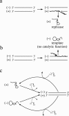
Figure 1
Figure 1
A scheme of self-replicating RNA with strand displacement. a and b show the two possible outcomes for replication from a double-stranded RNA by strand displacement. The single-stranded (+) catalyzes replication reactions, and is thus replicase. The single-stranded (-) carries no catalytic function. While it is arbitrary whether we designate single-stranded (+) strands or single-stranded (-) strands as replicases, the assumption that only one of the strands is the replicase is important. c shows the entire set of self-replication processes. Solid arrows represent replication reactions, where the origin of the arrows is the template and the end point of the affows is the product of replication. Dashed arrows represent catalysis. Note that both single-stranded (+) and (-) can serve as a template for replication, wherein replication gives rise to a double-stranded molecule.
Figure 2
Figure 2
Snapshots of simulations & population distribution of r. The right panels in each pair show a population distribution of r at a given time-step of simulations [where r = kDM/(kDM + kDP)]. Population distributions of r were observed after the system reached equilibrium. The abscissa is r in the range of [0,1] with 100 bins. The coordinate is the frequency of individuals (P or M or D) in the range of [0,0.1] (the sum of frequencies is normalized to 1). The left panels show the spatial distribution of individuals colored by value of r. Colors indicate values of r at the same time step as that of the population distribution of r (right panels). The values of the parameters are as follows: kSP = kSM = kDP + kDM = 1 (replication rates); d = 0.01 (decay rate); μ = 0.01 (mutation rate); δr = 0.1 (mutation step).
Figure 3
Figure 3
The evolution of strand preference (r) as a function of diffusion intensity (Δ). The population mean of r (r¯) is plotted as a function of the diffusion intensity (Δ) for various decay rates (d). Error bars show the mean absolute deviation of r in a population, which is defined as ADev(r) = ∑i|ri - r¯|/N where N is population size, and i denotes an individual. Both r¯ and ADev(r) were averaged over time after the system reached equilibrium. The other parameters than Δ and d are the same as in Fig. 2. For computational reason, the data for Δ = 100 are obtained from a field of 100 × 100 squares (note that diffusion will be effiectively stronger in a smaller field). The data for great values Δ are not plotted for d = 0.05 since the system goes extinct (this is because of the fluctuation in r¯, which is due to the system size being finite).
Figure 4
Figure 4
Advantage of producing (-) strands. The value of kP|ΣPP = (1 - e-(Δ+2a)τ)a/(Δ + 2a) (black solid line), that of kM|ΣMP = (1 - e-(Δ+a)τ)a/(Δ + a) (red dashed line) and the difference thereof (blue dotted line) are plotted as a function of Δ (τ is set to Δ-1), with a = 0.5 [a is the rate of replication for single stranded templates – either (+) or (-) strands]. For those plotted values to be applicable to the CA model, a should lie between 0.1kS and kS where kS = kSP = kSM. This is because in the CA model the number of neighbors are 8 (rather than 2), and these 8 neighbors are not necesarily all P. Thus, to calculate values corresponding to kP|ΣPP and kM|ΣMP in the CA model, one must also factor in the probability that a molecule (P or M) interacts with P given that they are in the neighborhood of the molecule (see Methods for the details of how interactions are implemented in the CA model).
Figure 5
Figure 5
The degree of spatial correlation within same species and between different species as a function of the density of observed species. n¯intra (circles) is the average number of molecules of the same species that a given molecule "meets" in a single time-step (i.e. that are in its neighborhood) (see main text for details). The abscissa (q) is the density of the same species, which is calculated as the number of individuals of that species divided by the total number of squares on the grid. n¯inter (crosses) is the average number of molecules of the opposite species that a given molecule meets in a single time-step. The abscissa (q) is the density of the opposite species, which is calculated in a manner similar to the case of n¯intra. The two species are identical with respect to the parameters, and both have r = 1/2. Colors represent diffusion intensity (Δ): Δ = 0.001 (black); Δ = 0.01 (red); Δ = 0.1 (green); Δ = 1 (blue). The rate of decay (d) is 0.05. Mutation is disabled (μ = 0). The other parameters are the same as in Fig. 2. A tentative explanation for why n¯intra is a linear function of q can be given as follows. Because of the local reproduction, when a species exists, it always exists on the grid as aggregates. Therefore, an individual always "meets" some number of individuals of the same species no matter what the density of the species in a whole system is (α > 0). When an aggregate "meets" with other aggregates, then the individuals will see more individuals of the same species, which increases n¯intra. Given that the aggregates are randomly distributed on the grid, the chance of an aggregate meeting with another aggregate is proportional to the number of aggregates in the system, which is proportional to the total density of the species (q). Therefore, n¯intra is a linear function of q. Because of the symmetry, n¯inter is also a linear function with the same slope as n¯intra (but the intercept must obviously be 0 for n¯inter.
Figure 6
Figure 6
Relationship between the critical degree of aggregation (α) and the sensitivity of correlation to the density of observed replicators (β). α and β are calculated as, respectively, the intercept and slope of the linear regression to n¯intra for intermediate values of q for which n¯intra is approximately linear to q (see Fig. 5). Values of d are as shown in the plot. For the same value of d, several data points are plotted for different values of Δ (from right to left, Δ = 0.0001, 0.001, 0.01, 0.1, 1, 10; points are almost on top of each other for Δ = 1 and 10). The other parameters are the same as in Fig. 5. Note that α can also be calculated from n¯inter since n¯inter has almost the same slope as that of n¯intra, as shown in Fig. 5. Also note that when α ≈ 0 (i.e. when Δ ≫ 1), β becomes almost 8 because the current CA model uses Moore (8) neighbors.
Figure 7
Figure 7
Advantage of producing (+) strands: the critical degree of aggregation (α) as a function of the diffusion intensity (Δ). α is plotted as a function of Δ by using the data of Fig. 6. This figure shows that the characteristic value of α for which a decreases depends on the value of d.
Figure 8
Figure 8
The effect of decay on the spatial distribution of replicators. Snapshots of simulations show a spatial distribution of replicators for different decay rates (d). The two colors represent two different "species", which have identical parameters (see "Multi-scale analysis of the model" under Results for more details). The intensity of diffusion (Δ) is 0.01. The other parameters are the same as in Fig. 5. The snapshots are taken when the frequency of two species is almost fifty-fifty. This figure shows that a greater decay rate (shorter longevity) of replicators leads to a greater spatial correlation within the same species.
Figure 9
Figure 9
Speciation: emergence of replicase transcribers (r ≈ 1) and parasitic genome copiers (r ≈ 0). This figure shows the results of a simulation where kSM and kSP can also evolve the correlation with kDM and kDP is not presumed, but it may evolve. The right panel shows a population distribution of r. The abscissa is r in the range of [0,1] with 100 bins. The coordinate is the frequency of individuals in the range of [0,0.25]. A bimodal distribution indicates a speciation-like phenomenon [the population distribution of kSP/(kSP + kSM) also shows a similar bimodal distribution; data not shown]. The left panel shows the spatial distribution of individuals colored by value of r. The color coding is the same as in the right panel (note that the color coding is different from that of Fig. 2). For the sake of comparison, the size of the grid is set to 300 × 300 as in Fig. 2. The parameters are as follows: 0.5(kSM + kSP) = (kDM + kDP) = 1; Δ = 0.01; d = 0.01; μ = 0.01; δr = 0.1. The mutation of kSM and kSP is implemented in the same way as that of kDM and kDP. [Additionaly, we observed the speciation-like phenomenon also in the following parameter conditions: d = 0.001 and 0.1 ≤ Δ ≤ 0.32; d = 0.01 and 0.001 ≤ Δ ≤ 0.1; d = 0.02 and Δ = 0.1.].
Figure 10
Figure 10
The evolution of strand preference (r) as a function of the diffusion intensity (Δ) in the system with complex formation. Solid lines represent the evolved value of r¯ as a function of the diffusion intensity (Δ) for various decay rates (d). Dashed lines represent the minimum value of r necessary to ensure system survival (rmin). Colors (and simbols) represent the value of d: d = 0.0025 (black circles); d = 0.0125 (red squares); d = 0.025 (blue triangles). The other parameters are as follows: kSP = kSM = kDP + kDM = 1; b = 1; κ = 1; μ = 0.01; δr = 0.1.

Similar articles

Cited by

References

    1. Bartel DP. In: The RNA world. 2. Gesteland RF, Cech TR, Atkins JF, editor. Cold Spring Harbor:Cold Spring Harbor Laboratory Press; 1998. Re-creating an RNA replicase; pp. 143–162.
    1. Kováč L, Nosek J, Tamáška L. An overlooked riddle of life's origins: energy-dependent nucleic acid unzipping. J Mol Evol. 2003;57:S182–S189. doi: 10.1007/s00239-003-0026-z. - DOI - PubMed
    1. Epstein IR. Competitive coexistence of self-reproducing macromolecules. J Theor Biol. 1979;78:271–298. doi: 10.1016/0022-5193(79)90269-8. - DOI - PubMed
    1. Biebricher CK, Eigen M, Gardiner WC Jr. Kinetics of RNA replication: competition and selection among self-replicating RNA species. Biochemistry. 1985;24:6550–6560. doi: 10.1021/bi00344a037. - DOI - PubMed
    1. Szathmáry E, Gladkih I. Sub-exponential growth and coexistence of non-enzymatically replicating templates. J Theor Biol. 1989;138:55–58. doi: 10.1016/S0022-5193(89)80177-8. - DOI - PubMed

Publication types

Substances

LinkOut - more resources