. 2008 Jul 11;4(7):e1000108.
doi: 10.1371/journal.pcbi.1000108.

Unraveling protein networks with power graph analysis

Affiliations

Unraveling protein networks with power graph analysis

Loïc Royer et al. PLoS Comput Biol. .

Abstract

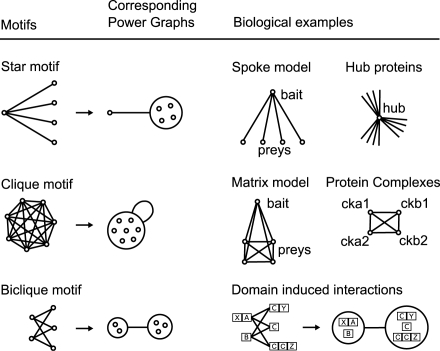
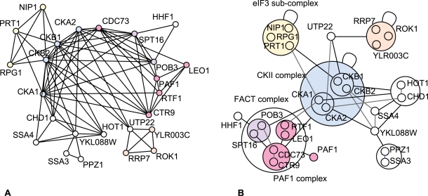
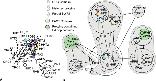
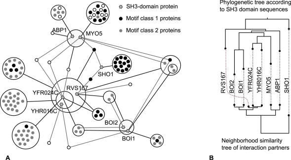
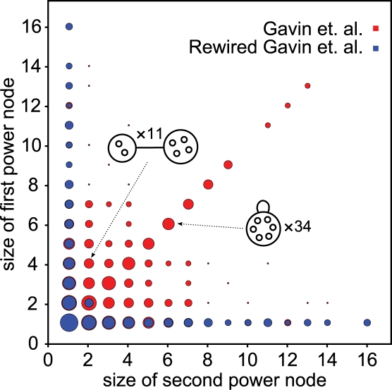
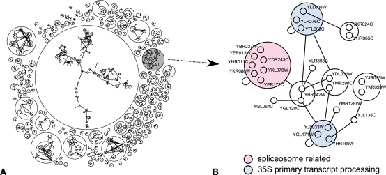
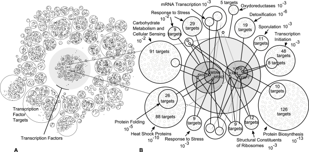
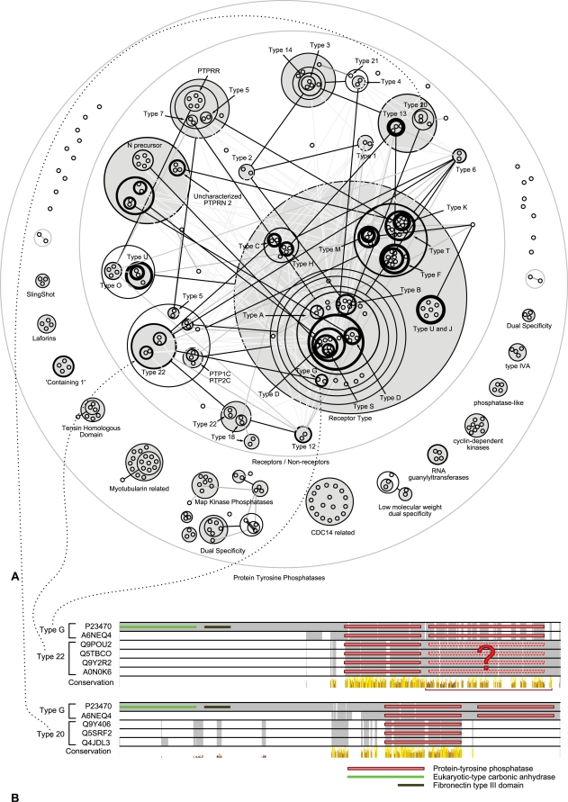
Networks play a crucial role in computational biology, yet their analysis and representation is still an open problem. Power Graph Analysis is a lossless transformation of biological networks into a compact, less redundant representation, exploiting the abundance of cliques and bicliques as elementary topological motifs. We demonstrate with five examples the advantages of Power Graph Analysis. Investigating protein-protein interaction networks, we show how the catalytic subunits of the casein kinase II complex are distinguishable from the regulatory subunits, how interaction profiles and sequence phylogeny of SH3 domains correlate, and how false positive interactions among high-throughput interactions are spotted. Additionally, we demonstrate the generality of Power Graph Analysis by applying it to two other types of networks. We show how power graphs induce a clustering of both transcription factors and target genes in bipartite transcription networks, and how the erosion of a phosphatase domain in type 22 non-receptor tyrosine phosphatases is detected. We apply Power Graph Analysis to high-throughput protein interaction networks and show that up to 85% (56% on average) of the information is redundant. Experimental networks are more compressible than rewired ones of same degree distribution, indicating that experimental networks are rich in cliques and bicliques. Power Graphs are a novel representation of networks, which reduces network complexity by explicitly representing re-occurring network motifs. Power Graphs compress up to 85% of the edges in protein interaction networks and are applicable to all types of networks such as protein interactions, regulatory networks, or homology networks.


Conflict of interest statement

The authors have declared that no competing interests exist.

Figures

Figure 1
Figure 1. The Three Basic Motifs: Star, Biclique, and Clique.
Stars often occur because of hub proteins or when affinity purification complexes are interpreted using the spoke model. Bicliques often arise because of domain-domain or domain-motif interactions inducing protein interactions . Power nodes are sets of nodes and power edges connect power nodes. A power edge between two power nodes signifies that all nodes of the first set are connected to all nodes of the second set. Note that nodes within a power node are not necessarily connected to each other.
Figure 2
Figure 2. Casein Kinase II Complex.
Two catalytic alpha subunits (CKA1, CKA2) and two regulatory beta subunits (CKB1, CKB2) interacting with the FACT complex, with sub-complex NIP1-RPG-PRT1, and with the PAF1 complex. The graph representation (A) consists of 80 edges whereas the power graph representation (B) has 30 power edges, thus an edge reduction of 62%. This simplification of the representation makes the separation of the regulatory subunits from the catalytic subunits immediately apparent without loss of information on individual interactions.
Figure 3
Figure 3. Histone Protein Interactions and Neighbouring Proteins according to Krogan et al. .
(A) Standard graph representation. (B) power graph representation. The ORC complex is visible with a power node of proteins–ORC1/ORC4/ORC5–carrying a nucleotide binding P-loop domain [SCOP:52540]. Histones subtypes HTA1/2, HTB1/2, HHT1/2, and HHF1/2 share the same color. Histones HTA2, HTB2 and HHF1 are segregated from their twin subtypes HTA1, HTB1 and HHF2. The FACT complex SPT16/POB3 is again delineated.
Figure 4
Figure 4. Interactions of SH3 Carrying Proteins.
(A) Protein interaction network showing the 105 interaction partners of the SH3 domain carrying proteins: SHO1, ABP1, MYO5, BOI1, BOI2, RVS167, YHR016C and YFR024. The underlying network consists of 182 interactions represented here as 36 power edges–a reduction of 80%–leaving all but only the core information. Class 1 motif (RxxPxxP) proteins are shown in black. Class 2 motif (PxxPxR) proteins are shown in light grey . Note how power graphs group proteins having similar binding motifs together. (B) Phylogeny and interaction profiles. Comparison of the phylogenetic tree of the SH3 domains sequences with the neighbourhood similarity tree of interaction partners. The neighbourhood similarity implied by the power graph reflects the sequence similarity of the SH3 domains.
Figure 5
Figure 5. Comparison of 13 Protein Interaction Networks to Corresponding Randomly Rewired Networks.
The edge reduction of the rewired networks is represented using a a box-plot. 50% of edge reduction values are inside the box. Most networks exhibit a significant deviation from the null model as indicated by high z-scores between 2.2 and 242.
Figure 6
Figure 6. Stars, Bicliques, and Cliques Counts as Obtained through Power Graph Analysis.
The area of each disc is proportional to the logarithm of the number of corresponding cliques (diagonal) and bicliques (non-diagonal). Stars are found along the first column or row. For example, there are 11 bicliques between two nodes and 4 nodes, and 34 bicliques of 6 nodes. The diagram is symmetric along the diagonal. Protein interaction networks from Gavin et al. (red) compared to corresponding rewired networks (blue). The high z-score (242) can be explained by significant abundance of cliques and bicliques compared to a random null-model obtained through rewiring. Note that despite the fact that the number of edges is constant, the total count of cliques, bicliques, and stars, is not necessarily constant.
Figure 7
Figure 7. Structural Interaction Network (SIN).
(A) Close-up of a 25 node, 68 edges, connected component of the Structural Interaction Network (SIN) . (B) Power graph consisting of 17 power edges, thus an edge reduction of 73%. Three cliques enriched in GO terms related to 35S primary transcript processing and to the spliceosome become explicit in the representation.
Figure 8
Figure 8. Examples of Occurrences of Bicliques in Gene Regulatory Networks and Homology Networks.
Bicliques can occur in regulatory networks due to two reasons: some transcription factors operate within complexes–combinatorial regulation–and regulatory motifs in promoter regions can be shared and repeated for different genes. In the case of homology networks, proteins sharing a sequence region of high similarity–i.e. a domain–induce cliques. Bicliques are similarly induced between sub-groups of similar proteins due additional region of sequence similarity.
Figure 9
Figure 9. Power Graphs Analysis of a Transcription Regulation Network.
(A) Power node hierarchy of the complete bipartite network between 158 transcription factors and 4217 target genes consisting of 13239 assignments between them. (B) Gene targets landscape of a group of transcription factors–SKN7, MSN2, MSN4, YAP1, YAP2(CAD1), and YAP7–regulating the general stress response of S. cerevisiae. Target genes are grouped within power nodes and linked with power edges signifying the assignment of transcription factors to targets. Dominant GO categories in target gene sets are indicated with the order of magnitude of the p-value.
Figure 10
Figure 10. Power Graph Analysis of the Human Protein Tyrosine Phosphatase Homology Network.
(A) The original homology network has 279 nodes and 4849 edges. The power graph has 209 power edges - with the addition of 95 non-singleton power nodes. Each node represents a human protein tyrosine phosphatase, with an edge between two proteins corresponding to highly significant alignments with E-values of at most 10−46. The network is obtained by an all against all BLASTP scan using the NCBI BLASTP tool . Greyed power nodes correspond to totally connected sets of proteins, for example, all receptor type protein tyrosine phosphatases have an alignment E-value of at least 10−46. Black power edges represent many edges of low E-values (lower than 10−46), light-gray power edges abstract fewer edges and correspond to less significant sequence similarities. (B) Multiple sequence alignment for type G against type 22 and type G against type 20. The similarity observed in the power graph between type G and type 22 is explained by the homology between a region of type 22 non-receptors and the second copy of the tyrosine phosphatase domain of type G receptors. Negative control: type G and type 20 - which are not linked - do not share this similar region.
Figure 11
Figure 11. Robustness of Power Graph Analysis through Random Rewiring.
Noise level is defined as the number of edges different from the original networks. Random rewiring leaves the total number of edges unchanged, thus a noise level of 100% means that all edges have changed. (A) Comparison of the power node hierarchies. The F1-measure of the precision and recall is computed between the power nodes found for the original network, and power nodes found for the rewired networks. (B) Comparison of the proximity of nodes in the power node hierarchies. Recall is obtained by comparing pairs of nodes together in a power node with the corresponding pairs of nodes in the power graph after random rewiring, the more distant in the power node hierarchy the lower the recall. Precision is obtained by starting from pairs of nodes together in power nodes found in the rewired networks and looking how far–in the power node hierarchy–are the corresponding nodes in the original network. The F1-measure of precision and recall is reported.
Figure 12
Figure 12. Power graph algorithm.
First a neighbourhood similarity clustering of the nodes is performed providing candidate power nodes. In a second step power edges are searched between nodes and candidate power nodes. Note that modular decomposition would not consider as a module the set of nodes having similar but non-identical neighbourhoods. The power graph algorithm finds this candidate and uses it to succinctly represent the biclique.
Figure 13
Figure 13. Scalability of Power Graph Analysis.
(A) Edge reduction versus edge density. Edge reduction attains a minimum for an edge density between 0.1 and 0.2 and the raises linearly (B) Edge to power node conversion rate versus edge density.

Similar articles

Cited by

References

    1. Fields S, Song O. A novel genetic system to detect protein-protein interactions. Nature. 1989;340:245–246. Available: http://dx.doi.org/10.1038/340245a0. - DOI - PubMed
    1. Rigaut G, Shevchenko A, Rutz B, Wilm M, Mann M, et al. A generic protein purification method for protein complex characterization and proteome exploration. Nat Biotechnol. 1999;17:1030–1032. Available: http://dx.doi.org/10.1038/13732. - DOI - PubMed
    1. Mann M, Hendrickson RC, Pandey A. Analysis of proteins and proteomes by mass spectrometry. Annu Rev Biochem. 2001;70:437–473. Available: http://dx.doi.org/10.1146/annurev.biochem.70.1.437. - DOI - PubMed
    1. Gavin AC, Aloy P, Grandi P, Krause R, Boesche M, et al. Proteome survey reveals modularity of the yeast cell machinery. Nature. 2006;440:631–636. Available: http://dx.doi.org/10.1038/nature04532. - DOI - PubMed
    1. Ito T, Chiba T, Ozawa R, Yoshida M, Hattori M, et al. A comprehensive two-hybrid analysis to explore the yeast protein interactome. Proc Natl Acad Sci U S A. 2001;98:4569–4574. Available: http://dx.doi.org/10.1073/pnas.061034498. - DOI - PMC - PubMed

Publication types

MeSH terms

Substances