. 2007 Sep 27;8 Suppl 6(Suppl 6):S9.
doi: 10.1186/1471-2105-8-S6-S9.

Current approaches to gene regulatory network modelling

Affiliations

Current approaches to gene regulatory network modelling

Thomas Schlitt et al. BMC Bioinformatics. .

Abstract

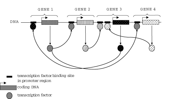
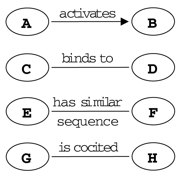
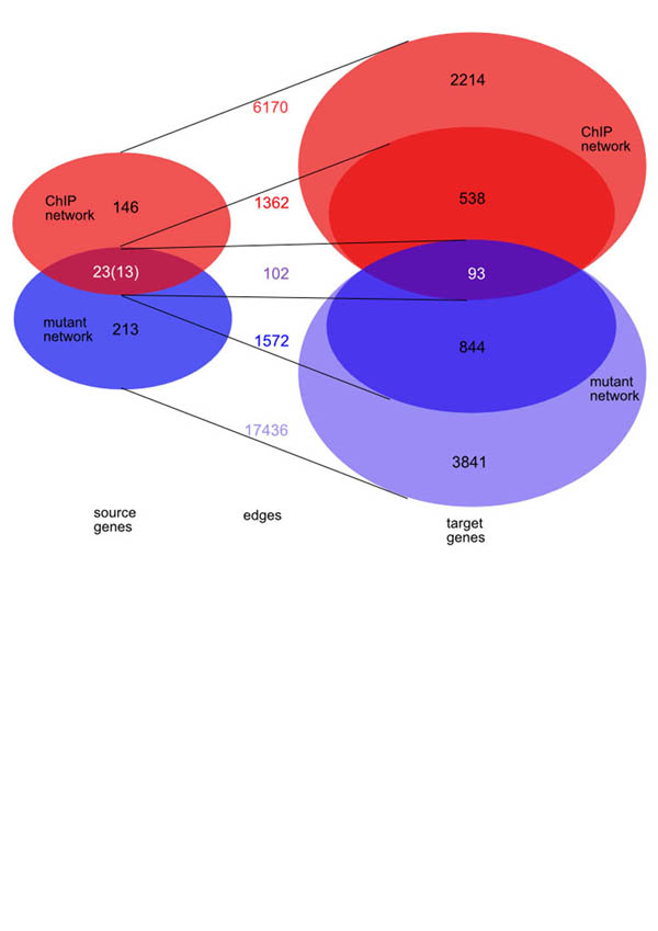
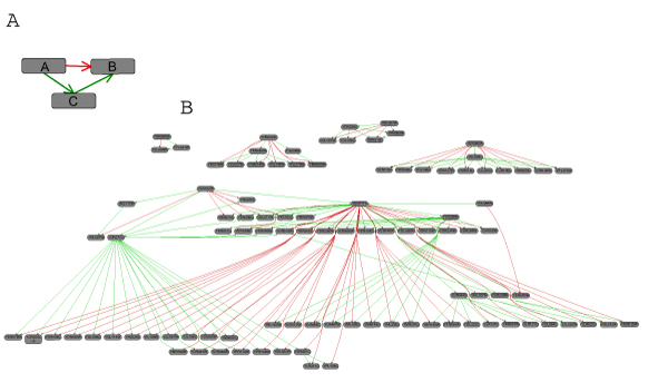
Many different approaches have been developed to model and simulate gene regulatory networks. We proposed the following categories for gene regulatory network models: network parts lists, network topology models, network control logic models, and dynamic models. Here we will describe some examples for each of these categories. We will study the topology of gene regulatory networks in yeast in more detail, comparing a direct network derived from transcription factor binding data and an indirect network derived from genome-wide expression data in mutants. Regarding the network dynamics we briefly describe discrete and continuous approaches to network modelling, then describe a hybrid model called Finite State Linear Model and demonstrate that some simple network dynamics can be simulated in this model.


Figures

Figure 1
Figure 1
Representation of a simple, fictional transcription factor network. All genes shown encode transcription factors that control the activity of genes encoding transcription factors.
Figure 2
Figure 2
Edges and arcs of a graph can represent different kinds of relationships. Some examples are shown.
Figure 3
Figure 3
Log-log plot of the node connectivity in different topological networks. The genes with the highest degrees are ABF1 in the ChIP-network and TUP1 in the mutant network, adapted from [2]
Figure 4
Figure 4
Venn diagrams of the intersection between the mutant and the ChIP network. The Venn diagram on the left hand side shows the intersection of the source genes between the mutant network and the ChIP network; the right hand side shows the intersections of the target genes between both networks. The connections between the two Venn diagrams indicate the corresponding number of edges. The networks share 23 source genes and 102 edges, but only 13 of the shared genes contribute to 102 shared edges, which connect to 93 distinct target genes. The 23 shared source genes are connected by 1362 edges to 631 target genes in the ChIP network and by 1572 edges to 937 target genes in the mutant network (see also Table 3).
Figure 5
Figure 5
Illustration of the target set comparison. A In the ChIP network transcription factors are connected to their target genes (regulation set); in the mutant network the deleted genes are linked to all genes with differential expression in this particular mutant background (effectual set). B Some transcription factors are present in both networks (ChIP and mutant network); we can therefore compare the genomic localisation (regulation set) with the expression changes in the mutant cell (effectual set). Reproduced from [2]
Figure 6
Figure 6
Direct and indirect effects. Red arcs are from the mutant network, green arcs from the ChIP network. A In the mutant where transcription factor A is deleted (disrupted) the expression of gene B is significantly different from its expression in the wild type. The transcription factor A does not bind to the putative promoter region of gene B (no green arc), but to the putative promoter region of transcription factor C, which in turn is found in the putative promoter region of gene B. This indirect path from A to B in the ChIP network might therefore explain the direct path in the mutant network. B All direct effects in the mutant network that could be explained by indirect paths via one additional transcription factor in the ChIP network.
Figure 7
Figure 7
Example for network logics. Genes A, B and C control the activity of gene D; D is active if A and B are bound, but not C; right: shows the FSLM representation for such a promoter. Reproduced from [2].
Figure 8
Figure 8
Decision trees. A decision tree is a special type of tree where the root and each interior node correspond to a variable; an arc to a child represents a possible value of that variable. A leaf represents the predicted value of target variable given the values of the variables represented by the path from the root. Following a route from the root node to a leaf node at each interior node we have to decide, which path to follow. Effectively each possible path encodes a decision rule. A Example for a decision tree. By following from the root node (top) to a leaf node (bottom) one has to make a decision at every interior node. B Corresponding set of decision rules.
Figure 9
Figure 9
Example for a small Boolean network consisting of 3 genes X, Y, Z. There are different ways for representing the network: A as a graph, B Boolean rules for state transitions, C a complete table of all possible states before and after transition, or D as a graph representing the state transitions. Reproduced from [2].
Figure 10
Figure 10
A metabolic reaction (left) and its representation as a Petri net (right). Aldolase splits one molecule of Fructose-1,6-bisphosphate into one molecule Dihydroxyacetonephosphate and one molecule Glyceraldehyde-3-phosphate. The Triosephosphateisomerase then transforms one molecule Dihydroxyacetonephosphate into one molecule Glyceraldehyde-3-phosphate (the reversibility of the reaction has been omitted here for the sake of clarity). In the Petri net representation place nodes (circles) are denoted by p, transition nodes (boxes) by t and tokens numbers by m. The place node p1 represents Fructose-1,6-bisphosphate and m1 the number of tokens or number of Fructose-1,6-bisphosphate molecules present. The transition node t1 represents the enzyme Aldolase. The weights on the edges reflect the stoichiometry of the reactions. p2 Dihydroxyacetonephosphate, m2 number of Dihydroxyacetonephosphate molecules, t2 Triosephosphateisomerase, p3 Glyceraldehyde-3-phosphate, m3 number of Glyceraldehyde-3-phosphate molecules.
Figure 11
Figure 11
The building blocks of the finite state linear model. A Binding sites are represented by triangles, control functions by boxes and substance generators by diamonds. Dotted lines represent cases where the discrete output of one element is the input for another element. B Switching behaviour of the binding sites. The curve (left) is typical for processes with hysteresis characteristics of a system that does not instantly follow the forces applied to it, but reacts slowly, or does not return completely to their original state: that is, systems whose states depend on their immediate history. The threshold for switching the states of the binding sites in FSLM is state dependent and results in a similar curve (right). [c] concentration of substance binding to binding site j; assoj, dissoj association and dissociation constants for binding site j; u binding site not occupied, o binding site occupied. Reproduced from [2].
Figure 12
Figure 12
Example for the dynamics of a simple FSLM network. A In this negative feedback loop the substance generator produces a substance, which acts as a repressor of its own control function. B Environment change graph recording the changes in repressor concentration during time. From the initial concentration the repressor accumulates with rate r+ until the association constant of the binding site brep is reached at time t1. Then the substance generator is switched off and the repressor degrades with rate r- until the dissociation constant is reached at time t2. The substance generator then produces the repressor until the association constant is reached again (means Boolean „not“). Reproduced from [2].
Figure 13
Figure 13
A FSLM network consisting of two genes and four binding sites. Left: The control functions of both genes have two inputs each. One input is from a binding site for its own substance, thus each gene is autoregulated by a negative feedback loop. Gene 1 has an additional negative feedback on gene 2, whilst gene 2 has an additional positive feedback on gene 1. Right: Result of the simulation of this network in FSLM. a1 association constantof binding site 1, d1 is the corresponding dissociation constant; a2, d2, a3, d3, a4, d4 correspondingly; ¬ Boolean „not“, &Boolean „and“. Reproduced from [2].
Figure 14
Figure 14
Description of phage λ using the elements of FSLM. In the FSLM model for phage λ the substance generators highlighted in grey produce substances, which bind to binding sites on the left (the connections have been omitted to improve the readability of the figure). The promoters PL1, PL2, PR1, and PR2 are used to model the behaviour of the λ terminator sites tL1, tL2, tR1, and tR2. The substance generators connected to them are only active, if N is bound to the respective binding sites. The substance "Struc" represents the structural proteins of the phage particles. The shaded grey boxes indicate the number of different states that the corresponding control functions can have. A simulation of phage λ using this model leads to lysogenic behaviour or lytic behaviour. In the lysogenic mode the initially active genes are inactivated, and the substance concentrations decrease rapidly, only CI is produced. The fluctuations of the CI concentration are due to the negative feedback loop involving the binding site OR3. In the lytic mode, CI and CII are not produced, but the other substance generators are active. The concentrations of Int, N, and Q increase infinitely because of the lack of a negative feedback control. The inset describes the effect of the stress response of the host cell using elements not yet implemented in the FSLM simulator. For a more detailed description of the model see [2, 91]. Reproduced from [2].

Republished from

Similar articles

Cited by

References

    1. Schlitt T, Brazma A. Modelling gene networks at different organisational levels. FEBS Lett. 2005;579:1859–1866. doi: 10.1016/j.febslet.2005.01.073. - DOI - PubMed
    1. Schlitt T, Brazma A. Modelling in molecular biology: describing transcription regulatory networks at different scales. Philos Trans R Soc Lond B Biol Sci. 2006;361:483–494. doi: 10.1098/rstb.2005.1806. - DOI - PMC - PubMed
    1. Ashburner M, Ball CA, Blake JA, Botstein D, Butler H, Cherry JM, Davis AP, Dolinski K, Dwight SS, Eppig JT, et al. Gene ontology: tool for the unification of biology. The Gene Ontology Consortium. Nat Genet. 2000;25:25–29. doi: 10.1038/75556. - DOI - PMC - PubMed
    1. Dandekar T, Schuster S, Snel B, Huynen M, Bork P. Pathway alignment: application to the comparative analysis of glycolytic enzymes. Biochem J. 1999;343:115–124. doi: 10.1042/0264-6021:3430115. - DOI - PMC - PubMed
    1. Pruess M, Fleischmann W, Kanapin A, Karavidopoulou Y, Kersey P, Kriventseva E, Mittard V, Mulder N, Phan I, Servant F, et al. The Proteome Analysis database: a tool for the in silico analysis of whole proteomes. Nucleic Acids Res. 2003;31:414–417. doi: 10.1093/nar/gkg105. - DOI - PMC - PubMed

LinkOut - more resources