. 2006 Apr 1;90(7):2344-55.
doi: 10.1529/biophysj.105.076778.

Inferring global topology from local juxtaposition geometry: interlinking polymer rings and ramifications for topoisomerase action

Affiliations

Inferring global topology from local juxtaposition geometry: interlinking polymer rings and ramifications for topoisomerase action

Zhirong Liu et al. Biophys J. .

Abstract

Lattice modeling is applied to investigate how the configurations of local chain juxtapositions may provide information about whether two ring polymers (loops) are topologically linked globally. Given a particular juxtaposition, the conditional probability that the loops are linked is determined by exact enumeration and extensive Monte Carlo sampling of conformations satisfying excluded volume constraints. A discrimination factor fL, defined as the ratio of linked to unlinked probabilities, varies widely depending on which juxtaposition is presumed. /log fL/s that are large for small loop size n tend to decrease, signaling diminishing topological information content of the juxtapositions, with increasing n. However, some juxtaposition geometries can impose sufficient overall conformational biases such that /log fL/ remains significant for large n. Notably, for two loops as large as n=200 in the model, the probability that passing the segments of a hooked juxtaposition would unlink an originally linked configuration is remarkably high, approximately 85%. In contrast, segment-passage of a free juxtaposition would link the loops from an originally unlinked configuration more than 90% of the time. The statistical mechanical principles emerging from these findings suggest that it is physically possible for DNA topoisomerases to decatenate effectively by acting selectively on juxtapositions with specific "hooked" geometries.


Figures

FIGURE 1
FIGURE 1
Three special 5 mer-on-5 mer juxtapositions configured on the simple cubic lattice: (I) hooked, (II) free (planar), and (III) free (nonplanar). They will be referred to by these labels throughout this study. Besides these three, many other juxtaposition geometries are possible in our model (Table 1). For every such juxtaposition, the middle positions of the two polymer chain segments are required to be nearest lattice neighbors (indicated by dashed lines connecting the two middle beads for the examples shown). Two-loop configurations are constructed by joining points i and ii with a self-avoiding lattice walk to form one ring polymer, and by joining points iii and iv by another self-avoiding walk to form a second ring polymer. To enforce excluded volume, every site on the lattice is not allowed to be occupied by more than one polymer element.
FIGURE 2
FIGURE 2
Schematics of two-loop configurations with different linking numbers Lk: (a) Lk = 0, (b) Lk = 1, and (c) Lk = 2. (d) Drawing of a lattice realization of two Lk = 2 loops with sizes n = 16. Lattice sites along the two different loops are represented, respectively, by white and black beads. Ten lattice sites constituting a hooked juxtaposition are marked by center black dots for the white beads and center white dots for the black beads. To elucidate the decatenation action of type 2 topoisomerases, the lattice chains here may be viewed as a model for the DNA double helix. This treatment does not address the internal structure of the DNA double helix, i.e., single-strand DNA is not considered. Accordingly, it should be noted that the loop-linking number Lk in this study does not correspond to the linking number defined for individual DNA strands.
FIGURE 3
FIGURE 3
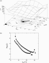
Discrimination factor fL (ratio of linked/unlinked number of configurations) of the hooked juxtaposition (Fig. 1, I) is determined by exact enumeration for two n = 16 loops. (a) fL as a function of the number of intraloop contacts within one (q11) and the other (q22) loops. fL is defined only at integer values of q11 and q22. The contour plot is constructed by interpolation for illustrative purposes. Areas on the q11q22 contour plot with highest values of fL are highlighted by shading: 1200 < fL < 1400 is in gray, and 1400 ≤ fL < 1600 is in black. (b) fL as functions of the number of interloop contacts q12 (•) or the total number of contacts q (▪, q = q11 + q12 + q22). Line segments joining data points are merely a guide for the eye. The minimum possible value of q is 5 because there are 5 interloop contacts in the hooked juxtaposition to begin with. Because there is no unlinked configuration for q = 5 when n = 16, formula image
FIGURE 4
FIGURE 4
Discrimination factors fL of the juxtapositions in Fig. 1 as functions of loop size n. Circles, squares, and triangles are, respectively, data points for the (I) hooked, (II) free (planar), and (III) free (nonplanar) juxtapositions in Fig. 1. Included for comparison is fL for a control situation (⋄) in which a pair of positions, one from each of the two loops (satisfying excluded volume conditions as before), are nearest neighbor on the lattice, but otherwise are not constrained. Thus, the diamonds in the plot correspond to the discrimination factor for a 1 mer-on-1 mer juxtaposition. In these plots, curves through the data points are a guide for the eye. Data for n ≤ 16 for the three 5 mer-on-5 mer juxtapositions and data for n ≤ 12 for the control are obtained by exact enumeration. Corresponding data for n ≥ 16 and n ≥ 12 are obtained by Monte Carlo sampling, with the number of attempted chain moves for each data point varying from 3 × 10⁹ to 1.8 × 10¹⁰.
FIGURE 5
FIGURE 5
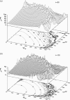
Discrimination factors of the hooked juxtaposition. Same as Fig. 3 but for larger loop sizes n = 50 (a) and n = 100 (b). Instead of using the exact enumeration method in Fig. 3, fL values in this figure are computed by Monte Carlo sampling from a total of 1.02 × 10¹² and 4.2 × 10¹¹ attempted chain moves, respectively, for n = 50 and n = 100. It should be noted that only q11 and q22 values that have been sampled are shown in these plots. Some large values of q11 and q22 were not encountered in the simulation because their probabilities are very small. The maximum possible values for either q11 or q22 are ≈58 for n = 50 and ≈136 for n = 100. The numbers 58 and 136 are the maximum possible numbers of contacts, respectively, for linear chains (53) with 50 and 100 beads. These numbers are upper bounds on the number of intraloop contacts here because for a given number of beads, any collection of loop conformations is a subset of all possible linear chain conformations.
FIGURE 6
FIGURE 6
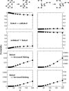
Changes of the linked/unlinked status of two-loop configurations caused by segment passage of different juxtapositions. The top graphics illustrate virtual segment-passages for a hooked (I) and a free (nonplanar, III) juxtaposition in the model. For each configuration obtained by exact enumeration or Monte Carlo sampling, a virtual segment passage operation at the given juxtaposition is performed to determine the resulting change in Lk. Four consequences of such topoisomerase-like processes are distinguished: i), a linked configuration becomes unlinked; ii), an unlinked configuration becomes linked; iii), the absolute value of the linking number of an originally linked configuration decreases, but the two loops remain linked; and iv), the absolute value of the linking number of a linked configuration increases. The probabilities of these four different outcomes are computed as functions of loop size n for an initially hooked (panels and scales on the left) or free (panels and scales on the right) juxtaposition. Since i–iv cover all possibilities, the probabilities for a given n along each vertical column add up to unity. Data for n ≤ 16 are obtained by exact enumeration; those for n ≥ 16 are from Monte Carlo sampling, where the number of attempted chain moves for each data point varies from 3 × 10⁹ to 1.8 × 10¹⁰. The maximum Lk encountered in our Monte Carlo simulations for the n = 200 loops here is Lk = 4 for the hooked juxtaposition and Lk = 3 for the free juxtaposition.
FIGURE 7
FIGURE 7
Schematics of a coarse-grained analytical description of juxtaposition geometry. (a) The curvature vector formula image of a 5 mer chain segment in this model is determined by the i – 2, i, and i + 2 positions: If i – 2, i, and i + 2 are collinear, formula image Otherwise, perpendicular bisectors of the line segment from i to i + 2, and of the line segment from i to i – 2 are constructed on the plane defined by i – 2, i, and i + 2. The radius of curvature R (notation not shown in the figure) is the magnitude of the vector from position i to the intersection point of the two perpendicular bisectors. formula image shares the direction of this vector but with 1/R as its magnitude. (b) The vectors formula image and formula image are the curvature vectors of two 5 mer polymer chain segments that make up a juxtaposition; formula image is the vector from the central position of the first 5 mer to the central position of the second 5 mer, and formula image Two scalar parameters are defined to characterize juxtaposition geometry in this study: formula image and formula image (see text for further details).
FIGURE 8
FIGURE 8
Schematics of representative juxtapositions belonging to different geometric regimes as defined by the parameters in Fig. 7.
FIGURE 9
FIGURE 9
Correlation between global topology and local juxtaposition geometry. The discrimination factors fL of all 2,982 possible 5 mer-on-5 mer juxtapositions are analyzed for loop sizes n = 14 (upper panels) and n = 50 (lower panels). (a and c) Scatter plots for formula image where juxtapositions with H ≥ 0 and H < 0 are represented, respectively, by open circles and solid dots. (b and d) Scatter plots for H, where juxtapositions with formula image and formula image are represented, respectively, by open circles and solid dots. The horizontal dashed lines mark the fL = 1 level, i.e., juxtapositions at this level have equal numbers of linked and unlinked two-loop configurations. Data for n = 14 in a and b are obtained by exact enumeration, whereas those for n = 50 in c and d are by Monte Carlo sampling using 5 × 10⁸ attempted chain moves for each data point. Large squares with incoming arrows marked by I, II, and III, are, respectively, data points for the hooked and free juxtapositions in Fig. 1. Data points for the free (nonplanar) juxtaposition (III) does not appear in the n = 14 plots because it is one of 32 juxtapositions with fL = 0 for n = 14 (and hence its formula image).

Similar articles

Cited by

References

    1. Sumners, D. W., and S. G. Whittington. 1988. Knots in self-avoiding walks. J. Phys. A.-Math. Gen. 21:1689–1694.
    1. Lickorish, W. B. R. 1997. An Introduction to Knot Theory. Springer-Verlag, New York.
    1. Buck, G. 1998. Four-thirds power law for knots and links. Nature. 392:238–239.
    1. Gambini, R., and J. Pullin. 2000. Loops, Knots, Gauge Theories and Quantum Gravity. Cambridge University Press, Cambridge, UK.
    1. Ladd, A. M., and L. E. Kavraki. 2004. Using motion planning for knot untangling. Int. J. Robot Res. 23:797–808.

Publication types

LinkOut - more resources