

Abstract
Genetic methods available in mice are likely to be powerful tools in dissecting cortical circuits. However, the visual cortex, in which sensory coding has been most thoroughly studied in other species, has essentially been neglected in mice perhaps because of their poor spatial acuity and the lack of columnar organization such as orientation maps. We have now applied quantitative methods to characterize visual receptive fields in mouse primary visual cortex V1 by making extracellular recordings with silicon electrode arrays in anesthetized mice. We used current source density analysis to determine laminar location and spike waveforms to discriminate putative excitatory and inhibitory units. We find that, although the spatial scale of mouse receptive fields is up to one or two orders of magnitude larger, neurons show selectivity for stimulus parameters such as orientation and spatial frequency that is near to that found in other species. Furthermore, typical response properties such as linear versus nonlinear spatial summation (i.e., simple and complex cells) and contrast-invariant tuning are also present in mouse V1 and correlate with laminar position and cell type. Interestingly, we find that putative inhibitory neurons generally have less selective, and nonlinear, responses. This quantitative description of receptive field properties should facilitate the use of mouse visual cortex as a system to address longstanding questions of visual neuroscience and cortical processing.
Keywords: visual cortex, receptive field, mouse, orientation, spatial frequency, contrast-invariant tuning
Introduction
Over the past nearly half century since visual responses were first described in the mammalian visual cortex (Hubel and Wiesel, 1962), there has been intensive research into the neural circuit and developmental mechanisms that give rise to selective receptive field (RF) properties. However, although the description of visual encoding has become increasingly more quantitative (Ringach, 2004; Carandini et al., 2005), as has the anatomy of neuronal subtypes (Gilbert, 1983; Douglas and Martin, 2004), it has been difficult to link these functional and anatomical findings into a local circuit model of cortical processing. Even more questions remain about how such a circuit might be assembled during development, despite advances in understanding the molecular mechanisms involved (Waites et al., 2005; Rash and Grove, 2006; Polleux et al., 2007) and the consequences of altered sensory input (Hensch, 2005; Hofer et al., 2006).
The recent proliferation of genetic technology in mice may provide tools to answer many of these questions (Callaway, 2005). Targeted gene disruption and transgene expression can result in much more specific manipulations than have been possible via pharmacology or sensory alteration and can allow perturbation of cellular signaling (Huang et al., 1999; Karpova et al., 2005), synaptic plasticity (Zeng et al., 2001; Sawtell et al., 2003), and firing patterns (Tan et al., 2006; Zhang et al., 2007a), even at the single-cell level (Brecht et al., 2004). Furthermore, fluorescent protein labeling provides precise anatomical techniques to yield information about cell type (Feng et al., 2000; Tamamaki et al., 2003) or even synaptic connectivity (Wickersham et al., 2007) in the intact brain, bridging the gap between circuit structure and function. Indeed, studies have already begun to take advantage of genetic methods to study visual system development (Fagiolini et al., 2003; Cang et al., 2005), plasticity (Fagiolini et al., 2004; Syken et al., 2006), and function (Sohya et al., 2007).
Studies of cortical visual processing have typically used carnivores or primates, which are considered to have a more refined visual system, including a much larger cortical region for visual processing, higher acuity, extensive visual behaviors, and orientation, ocular dominance, and spatial frequency columns (Issa et al., 2000; Ohki and Reid, 2007; Van Hooser, 2007). Understanding visual processing in such a simple system as the mouse cortex, which lacks both fine-scale spatial acuity and maps such as orientation columns, should provide insight into the minimal mechanisms necessary for receptive field development and function. However, although recent studies in rat and squirrel have described receptive field properties in the absence of orientation maps (Fagiolini et al., 1994; Girman et al., 1999; Heimel et al., 2005; Ohki et al., 2005), much less is known about visual encoding and processing in mice. Several early electrophysiology studies (Dräger, 1975; Mangini and Pearlman, 1980; Metin et al., 1988) (for review, see Hubener, 2003) indicated that, although mouse cortical neurons can be classified into categories similar to those described in other species, their overall level of stimulus selectivity may be significantly less than that of other species. However, these studies are difficult to evaluate because they were performed before many of the recent quantitative techniques for receptive field characterization were developed. A recent study, using two-photon imaging of calcium signals, measured differences in orientation selectivity in inhibitory and excitatory neurons of mouse primary visual cortex V1 (Sohya et al., 2007) but did not perform a thorough characterization of other visual responses and selectivity and was restricted to imaging the superficial layers.
We therefore undertook a quantitative survey of receptive field properties in V1 of the anesthetized mouse. In addition to determining the types of stimuli and range of stimulus parameters that are appropriate for probing vision in mice, we sought to confirm that the basic properties of visual processing that have been studied in other species are present in mice. These include orientation and spatial frequency tuning, the presence of both simple and complex response types, and higher-order properties such as contrast-invariant tuning. Furthermore, to relate these functional properties to computation in the cortical circuit, we analyzed responses by their laminar location within cortex and by putative identity as inhibitory versus excitatory neurons based on spike waveform.
Materials and Methods
In vivo physiology.
Recordings were made from adult C57BL/6 mice, 2–6 months of age. The animals were maintained in the animal facility at University of California, San Francisco (UCSF) and used in accordance with protocols approved by the UCSF Institutional Animal Care and Use Committee. For surgery, mice were sedated with an intraperitoneal injection of chlorprothixene (5 mg/kg) and then anesthetized with urethane (0.5–1.0 g/kg, i.p., at 10% w/v in saline). Administration of chlorprothixene several minutes before urethane greatly reduced the dosage of urethane necessary to induce surgical anesthesia. Additionally, atropine (0.3 mg/kg) and dexamethasone (2 mg/kg) were administered subcutaneously to reduce secretions and edema, respectively. The animal was maintained at 37.5°C by a feedback-controlled heating pad. A tracheotomy was performed, and a small glass capillary tube was inserted to maintain a free airway. After retracting the scalp, we performed a small craniotomy, ∼1 mm in diameter, and nicked a slit in the dura to allow insertion of the multisite electrode. The exposed cortical surface was covered with 2.5% agarose in extracellular saline (in mm: 125 NaCl, 5 KCl, 10 glucose, 10 HEPES, and 2 CaCl2, pH 7.4) to prevent drying and provide mechanical support. The electrode was lowered into the brain through the agarose to an appropriate depth and was allowed to settle for 30–45 min before the beginning of recording. The electrode was placed without regard for the presence of visually responsive units, and all units stably isolated over the recording period were included. For superficial recordings, the electrode was often inserted at an angle, to increase the distance between the insertion and recording sites. The eyes were covered with ophthalmic lubricant ointment until recording, at which time the eyes were rinsed with saline and a thin layer of silicone oil (30,000 centistokes) was applied to prevent drying while allowing clear optical transmission. We did not induce cycloplegia, and the resting pupil diameter was ∼1 mm. We recorded only at sites with receptive fields located at least 20° lateral to the visual meridian, to avoid confounding effects attributable to the binocular zone of vision.
At the end of recording, the animal was killed by overdose of barbiturates. For histology, the animal was intracardially perfused with 4% paraformaldehyde in PBS, and the brain was sectioned coronally at 100 μm with a vibratome (Lancer). Sections were incubated for several hours in 0.1 μg/ml 4′,6-diamidino-2-phenylindole (DAPI; Sigma-Aldrich) to stain nuclei and imaged on an epifluorescence microscope.
Recordings were made with silicon microprobes from NeuroNexus Technologies. Two configurations were used: a linear probe with 16 sites spaced at 50 μm intervals (model a1x16-3mm50-177), which could be used to span across multiple layers of cortex; and a tetrode configuration, with four tetrode clusters, each consisting of four sites separated by 25 μm on a side (model a2x2-tet-3mm-150-121), which was used primarily to provide better isolation of units in layers 2/3 and 4. Approximately two-thirds of all units were recorded with the tetrode configuration. The shanks of the probes were 15 μm thick and 3 mm long, with a maximum width at the top of the shank of 94 μm (tetrode) or 123 μm (linear.) For experiments followed by histology to reconstruct penetrations, the electrode was coated with a small amount of the lipophilic vital dye DiI (Invitrogen). Signals were acquired using a System 3 workstation (Tucker-Davis Technologies) and analyzed with custom software in Matlab (MathWorks). For local field potential (LFP) recording, the extracellular signal was filtered from 1 to 300 Hz and sampled at 1.5 kHz. Current source density (CSD) was computed from the average LFP by taking the discrete second derivative across the electrode sites, at two-site spacing to reduce noise, and interpolated to produce a smooth CSD map.
For single-unit recording, the extracellular signal was filtered from 0.7 to 7 kHz and sampled at 25 kHz. Spiking events were detected on-line by voltage threshold crossing, and a 1 ms waveform sample was acquired around the time of threshold crossing. To improve isolation of single units, recordings from groups of four neighboring sites were linked, so that a waveform was acquired on all four sites in response to a threshold crossing on any of the four. This procedure was used for both the tetrode and linear configuration electrodes; in the latter case, sites 1–4, 5–8, 9–12, and 13–16 (in order along the shank) were grouped together. In both cases, this “virtual tetrode” acquisition had two primary benefits: improved discriminability when a waveform appeared on more than one site, and common-mode noise rejection of signals shared on all four sites. Whereas the larger amplitude spikes of layer 5 and layer 6 units were sometimes recorded simultaneously on adjacent sites at the 50 μm spacing of the linear electrode, layer 2/3 neurons often appeared predominantly on one site, even at the 25 μm spacing of the tetrode configuration. In both cases, many units had signals on nondominant sites that were below the voltage trigger threshold; however, the simultaneous acquisition allowed this low-amplitude information to be integrated to improve discriminability.
The individual waveform samples were aligned by their most negative time point. To identify single units, the spike waveforms from the four sites together were parameterized by 6–10 independent components using the FastICA package for Matlab (http://www.cis.hut.fi/projects/ica/fastica/) and clustered by a mixture-of-Gaussians model using KlustaKwik (Harris et al., 2000). Using independent components, rather than principal components, allowed us to take advantage of common-mode noise rejection from waveforms simultaneously acquired across multiple sites in the virtual tetrode configuration. Whereas independent components analysis (ICA) has been used previously to filter the continuous data across channels (Snellings et al., 2006), we instead performed ICA on the individual waveforms, to integrate waveform parameterization and noise rejection. Quality of separation was determined based on the Mahalanobis distance and L-ratio (Schmitzer-Torbert et al., 2005) and the presence of a clear refractory period.
Units were then classified as narrow or broad spiking based on properties of their average waveforms, at the electrode site with largest amplitude. Three parameters were used for discrimination (Fig. 1 F,G): the height of the positive peak relative to the initial negative trough, the time from the minimum of the initial trough to maximum of the following peak, and the slope of the waveform 0.5 ms after the initial trough. This third measure provided a proxy for the total duration of the slower positive peak, because our waveform sampling was not of sufficient duration to measure the entire return to baseline. Two linearly separable clusters were found, corresponding to narrow-spiking (putative inhibitory) and broad-spiking (putative excitatory) neurons. These clusters were separated identically by both k-means and linkage clustering. Unit classification was stable and did not change when only two of the three measurements were used. The width of the initial trough, as used previously (Bruno and Simons, 2002), did not give good separation, which may be attributable to filtering by the electrodes or acquisition system because this is the shortest timescale in the waveform, or to its sensitivity to the alignment of individual waveforms in computing the average waveform. Because of the small numbers of narrow-spiking units in each layer, in cases in which no significant difference was seen across the individual layers, we pool together data for narrow-spiking units from all layers into one category for presentation.
Figure 1.
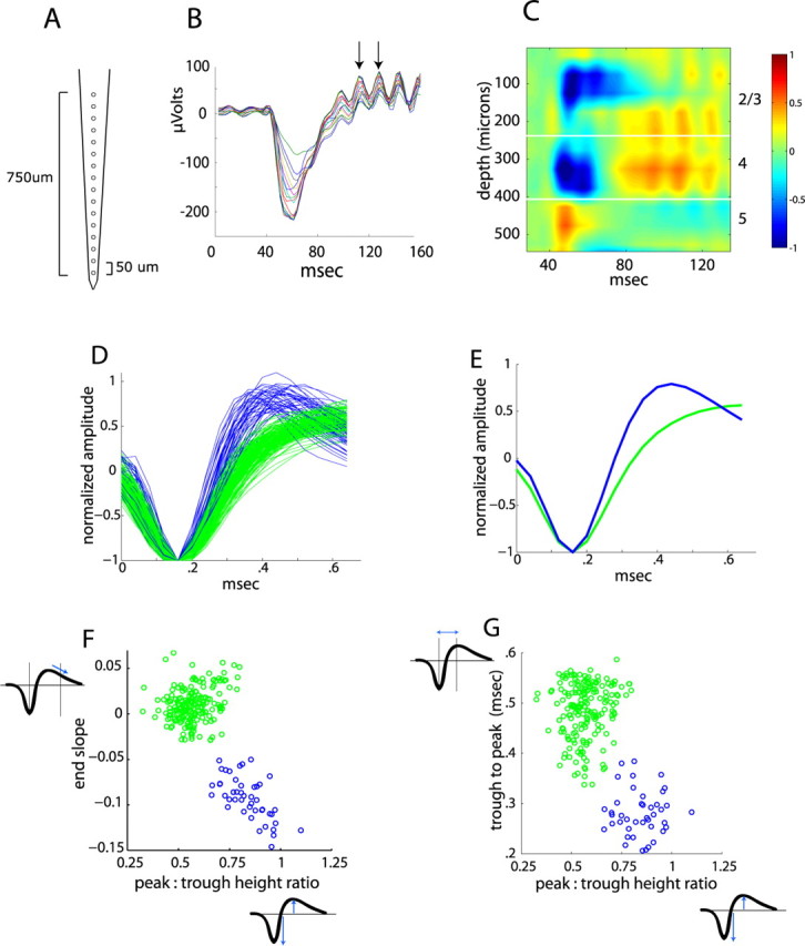
Laminar location and spike waveform classification. A, Schematic of linear multisite probe. B, Average LFP responses for 16 sites through the depth of cortex. Arrows show consecutive peaks of the high-frequency oscillation. C, CSD analysis of traces in B demonstrates segregation of responses by layer. Blue represents current sinks, and red represents current sources. Because the CSD is based on a second derivative at two-site spacing, the CSD cannot be computed for the top two and bottom two sites, so it spans 550 μm rather than 750 μm. Units for CSD are normalized from −1 to 1. D, Average spike waveforms for all units analyzed, aligned to minimum and normalized by trough depth, demonstrating narrow-spiking (blue; n = 45) and broad-spiking (green; n = 186) units. E, Average of all waveforms for narrow-spiking and broad-spiking units. F, G, Scatter plot of spike waveform parameters for all units.
Visual stimuli.
A challenge involved in our approach of unbiased recording from a number of neurons simultaneously is that stimuli cannot be tailored to individual neurons. For example, it is much faster to measure spatial frequency tuning of a single unit by finding the optimal orientation and then varying the spatial frequency only at this orientation than by presenting all orientations and all spatial frequencies, as in this study. This also limited our ability to vary multiple parameters in a single stimulus set: for example, to measure contrast-invariant tuning, we chose one spatial frequency and then varied orientation and contrast, because the curse of dimensionality makes it impractical to sample finely across all three parameters. Thus, the response was limited to those neurons tuned to the spatial frequency we chose. This will become even more of a limitation in new techniques, such as two-photon calcium imaging, which can sample large populations but have poorer temporal resolution. Stimuli similar to the contrast-modulated noise movies described below, which can provide rapid measures of responsiveness across a widely tuned population, may help to address these challenges.
Stimuli were generated in Matlab using the Psychophysics Toolbox extensions (Brainard, 1997; Pelli, 1997) and displayed with gamma correction on a monitor (Nanao Flexscan, 30 × 40 cm, 60 Hz refresh rate, 32 cd/m2 mean luminance) placed 25 cm from the mouse, subtending ∼60 × 75° of visual space. Episodic stimuli were repeated five to seven times, with stimulus conditions randomly interleaved, and a gray blank condition (mean luminance) was included in all stimulus sets to estimate the spontaneous firing rate.
Episodic stimuli included drifting sinusoidal gratings [1.5 s duration, temporal frequency of 2 Hz, 12 directions, spatial frequency of 0.01, 0.02, 0.04, 0.08, 0.16, 0.32, and 0 cycles/° (cpd), i.e., full-field flicker], full-length drifting bars (width of 5°, velocity of 30°/s, 16 directions), drifting short bars (4 × 8°, 30°/s, four directions), contrast-reversing (counter phase) sinusoidal gratings (0.04 cpd, sinusoidally reversing at temporal frequencies 1, 2, 4, and 8 Hz, eight orientations, 2 s duration), and contrast-reversing square checkerboard (0.04 cpd, square-wave reversing at 0.5 Hz). Episodic stimuli were shown at 100% contrast with the background at mean luminance, except in a subset of experiments on contrast-invariant tuning, in which drifting sinusoidal gratings were presented as described above but at fixed spatial frequency of 0.04 cpd and contrast 6.25, 12.5, 25, 50, and 100%.
Gaussian noise movies were created by first generating a random spatiotemporal frequency spectrum in the Fourier domain with defined spectral characteristics. To drive as many simultaneously recorded units as possible, we used a spatial frequency spectrum that dropped off as A(f) ∼ 1/(f + fc), with fc = 0.05 cpd, and a sharp cutoff at 0.12 cpd, to approximately match the stimulus energy to the distribution of spatial frequency preferences. The temporal frequency spectrum was flat with a sharp low-pass cutoff at 4 Hz. This three-dimensional (ωx, ωy, ωt) spectrum was then inverted to generate a spatiotemporal movie. This stimulus is related to the subspace reverse correlation method (Ringach et al., 1997), in that both explicitly restrict the region of frequency space that is sampled. To provide contrast modulation, this movie was multiplied by a sinusoidally varying contrast. Movies were generated at 60 × 60 pixels and then smoothly interpolated to 480 × 480 pixels by the video card to appear at 60 × 60° on the monitor and played at 30 frames per second. Each movie was 5 min long and was repeated two to three times, for 10–15 min total presentation. A brief clip of the contrast-modulate movie is available as supplemental data (available at www.jneurosci.org as supplemental material).
Data analysis.
The average spontaneous rate for each unit was calculated by averaging the rate over all blank condition presentations. For drifting gratings, responses at each orientation and spatial frequency were calculated by averaging the spike rate during the 1.5 s presentation and subtracting the spontaneous rate. The preferred orientation was determined by averaging the response across all spatial frequencies and calculating half the complex phase of the value
The orientation tuning curve was constructed for the spatial frequency that gave peak response at this orientation. Given this fixed preferred orientation θpref, the tuning curve was fitted as the sum of two Gaussians centered on θpref and θpref + π, of different amplitudes A 1 and A 2 but equal width σ, with a constant baseline B. From this fit, we calculated two metrics: an orientation selectivity index (OSI) representing the ratio of the tuned versus untuned component of the response, and the width of the tuned component. OSI was calculated as the depth of modulation from the preferred orientation to its orthogonal orientation θortho = θpref + π/2, as (R pref − R ortho)/(R pref + R ortho). Tuning width was the half-width at half-maximum of the fit above the baseline, R ortho. In addition, direction selectivity was calculated from the fitted function as (R pref − R opposite)/(R pref + R opposite).
We used these measures of selectivity, rather than the circular variance, because the circular variance, which is a single global measure of the tuning curve, combines aspects of both depth of modulation and tuning width into one value and thus does not give as intuitive a description of the tuning curve (but see Ringach et al., 2002 for a thorough exposition). Furthermore, because it has not yet gained common usage, there is less previous data for comparison. However, measuring orientation selectivity as (1 − circular variance), i.e., the absolute value of S as defined above, gave similar results (supplemental Fig. S2, available at www.jneurosci.org as supplemental material) and should be useful in the future, particularly in cases in which a single metric for orientation selectivity is desirable.
The spatial frequency tuning curve was determined from drifting gratings from the response at orientation θpref described above and was fit to a difference of two Gaussians (Hawken and Parker, 1987). Bandwidth was calculated from the fit as the ratio of the spatial frequencies that gave half-maximal response. Units were classified as having low-pass spatial frequency tuning if the response to 0 cpd, the full-field flicker, was at least 50% of the peak response.
Linearity of response was calculated from drifting gratings, at the orientation and spatial frequency that gave peak response. First, we binned the 1.5 s presentation into a spike histogram at 100 ms intervals and subtracted the spontaneous rate. We then applied the discrete Fourier transform and computed F 1/F 0, the ratio of the first harmonic (response at the drift frequency) to the 0th harmonic (mean response).
Responses to drifting full-field bars were analyzed by computing peristimulus time histograms with bin size 100 ms. The spontaneous rate was subtracted, and the peak firing rate for each orientation was used to generate an orientation tuning curve, which was fit to the sum of two Gaussians and analyzed as described above.
Receptive field size was calculated from 4 × 8° light bars. Bars were swept across the visual field at eight locations along the axis perpendicular to the direction of motion, e.g., for horizontally moving bars, each presentation swept a bar across at a different vertical position. The responses from the eight sweeps were binned at 100 ms and used to construct firing rate as a function of bar position. This was fitted with a two-dimensional Gaussian, with independent widths σx and σy, and RF radius was calculated by averaging the half-width at half-maximum of the two axes of the Gaussian fit (equivalent to the semi-major and semi-minor axes of the ellipse generated by the half-maximum contour). This process was repeated for four different directions and averaged across all conditions that gave a sufficient response. The bar length, 8°, was chosen to elicit strong responses from as many units as possible. However, it puts a lower limit on our measurement of RF size, ∼4°, so we may have overestimated the size of the smallest receptive fields.
Temporal frequency was calculated from the response to contrast-reversing sinusoidal gratings at a fixed spatial frequency of 0.04 cpd. The average firing rate over each 2 s presentation was calculated, and the spontaneous rate was subtracted. For the orientation that gave the largest total response, a temporal frequency tuning curve was fit using a difference of two Gaussians.
To analyze the response to contrast-modulated white noise movies, we binned the number of spikes in response to each frame of the movie. A responsiveness metric was calculated by taking the discrete Fourier transform at the modulation frequency, normalized by the average firing rate. Additionally, the spike-triggered average (STA) of contrast-modulated movie responses was computed by the mean of the frames preceding each spike. Because we used a 1/f power spectrum for the stimulus set, the raw STA is broadened by the correlations in the stimulus set. However, because the stimulus is Gaussian and therefore only contains second-order correlations, we were able to correct the STA exactly by normalizing its Fourier transform by the power spectrum of the stimulus set (Theunissen et al., 2001; Sharpee et al., 2004). In general, the strongest STAs preceded spikes by a lag of two movie frames (66 ms). Preferred orientation and spatial frequency were calculated by finding the peak of the spatial Fourier transform of the STA at 66 ms lag. STA receptive fields were also fit to Gabor functions (a sinusoid with a Gaussian envelope), described by
 |
where x′ and y′ are rotated, and translated coordinates are defined by x′ = cosθ(x − x c) + sinθ(y − yc) and y′ = −cosθ(x − x c) + cosθ(y − yc). Fits were performed in Matlab, based on routines provided by Michael Lewicki and colleagues.
Contrast–response curves were generated from the response to drifting gratings with spontaneous rate subtracted, for the preferred orientation determined as above. Because stimuli were presented at a preselected spatial frequency (0.04 cpd) rather than the preferred spatial frequency of each unit, the peak firing rate is not indicative of the maximal responsiveness of the unit, and the curves were thus normalized to maximum response of 1. Normalized curves were fit to the Naka–Rushton equation (Naka and Rushton, 1966): R(C) = g/(1 + (C/C 50)b), where C is contrast, g is the gain, C 50 is the midsaturation contrast, and b is a fitting exponent that describes the shape of the curve.
Statistical significance was determined by Mann–Whitney U test, except when otherwise stated. In the figures, *p < 0.05, **p < 0.01, and ***p < 0.001. For figures representing the median of data, error bars show standard error of the median as calculated by a bootstrap. In other cases, error bars represent SEM.
Results
Laminar and cell-type identity
We recorded 235 isolated single units from 27 adult mice. Individual recording sessions consisted of simultaneous recordings of ∼4–12 isolated single units across the 16 sites of the multielectrode array. Of these units, 87% (204 of 235) were responsive to at least one episodic visual stimulus. Nonresponsive units were not included in analysis of tuning properties. We generally performed only one electrode insertion per animal to avoid damage to cortex from multiple penetrations and to maintain a stable anesthetic state without needing to redose.
To verify the laminar location of each recording site of the multielectrode array, we measured in addition to electrode depth the LFP response to square-wave contrast reversal of a checkerboard. As shown in Figure 1 B, the averaged responses show a large deflection starting ∼40 ms after the contrast reversal, which varies in both amplitude and waveform across the recording sites. CSD analysis provides a method to transform the set of LFP recordings into the locations of current sources and sinks, with current sinks generally corresponding to sites of synaptic conductances (Mitzdorf, 1985; Swadlow et al., 2002). This transformation revealed a laminar distribution of activation in response to checkerboard reversal (Fig. 1 C), with a current sink beginning in layer 4, in which sensory input first arrives, spreading up to layer 2/3, and finally a weak sustained sink in layer 5. Retrospective histology (supplemental Fig. S1, available at www.jneurosci.org as supplemental material) confirmed the correspondence between CSD and laminar identity. Furthermore, layer 4 corresponded to the maximum negativity of initial dip in the LFP (Fig. 1 B,C) (supplemental Fig. S1, available at www.jneurosci.org as supplemental material), which allowed us to deduce the laminar location even for recordings that did not span the entire depth of cortex and therefore could not generate a full CSD map of the layers. As shown below, this assignment of layers correlates with different properties of the visual response. Furthermore, during recording, it was generally possible to recognize these laminar positions qualitatively by the nature of ongoing activity: layer 2/3 has very sparse background activity; in layer 4, the spontaneous rate increases and more units are present on each recording site; layer 5 has dramatically higher spontaneous rates and much larger spike amplitudes; and, in layer 6, spontaneous rates and spike amplitudes decrease and evoked responses are more sparse.
Interestingly, we often saw a fast oscillation, at ∼50–55 Hz, superimposed on the LFP and CSD (Fig. 1 B, arrows). This oscillation was stimulus evoked, with coherent activity commencing with the onset of the evoked LFP. Furthermore, its frequency spectrum was distinct from typical 60 Hz noise and did not change as we varied the refresh rate of the display. We thus presume that this corresponds to gamma oscillations that have been described in many species (Buzsáki and Draguhn, 2004), including mice (Nase et al., 2003). However, we did not investigate this oscillation further.
As an additional means of correlating visual responses with cortical circuit elements, we classified units based on their spike waveform. Figure 1 D shows the average waveforms from all the units recorded, except for four units that had unusual waveforms and were excluded from classification. The waveforms can be seen to fall into two general classes, narrow spiking (blue) and broad spiking (green), with averages across the two classes shown in Figure 1 E. Previous results have suggested that narrow-spiking cells correspond to inhibitory, predominantly fast-spiking, interneurons (McCormick et al., 1985; Connors and Kriegstein, 1986; Barthó et al., 2004), and recent studies have used this extracellular signature as a means of distinguishing excitatory and inhibitory neurons (Swadlow, 2003; Andermann et al., 2004; Lee et al., 2007; Mitchell et al., 2007; Atencio and Schreiner, 2008). A variety of waveform parameters have been used to separate these two classes, including trough-to-peak time (Barthó et al., 2004; Mitchell et al., 2007), the ratio of trough-to-peak amplitude (Andermann et al., 2004; Hasenstaub et al., 2005), and the duration of the longer, positive peak (Bruno and Simons, 2002; Atencio and Schreiner, 2008). Because our acquisition did not record the entire duration of the positive peak, we used the slope 0.5 ms after the initial trough (i.e., how quickly the voltage is returning to baseline) as a proxy for this parameter. These three parameters provided good separability and distinguished the same two groups of waveforms, as shown in Figure 1, F and G. Nineteen percent of the total population of recorded cells (45 units) fell into the narrow-spiking category, and there was not a significantly greater fraction of narrow-spiking units in any particular layer (p > 0.1, χ2 test). This proportion matches the fraction of GAD-positive neurons previously identified histochemically (Tamamaki et al., 2003). For simplicity, we refer to these two groups as “putative inhibitory” and “putative excitatory,” but this should not imply that there is a perfect correspondence between the spike waveform and cell type assignment (see Discussion).
Selective and nonselective responses
A characteristic of visual cortex responses is the transformation from primarily center-surround, nonoriented receptive fields observed in retina and lateral geniculate nucleus of thalamus (LGN), to responses in V1 that are optimal for bars and edges of a particular orientation. To measure the degree of orientation and other response selectivity in mouse visual cortex, we presented full-length 5° wide bars of varying orientations drifting at 30°/s and drifting sinusoidal gratings moving at 2 Hz of varying orientation and spatial frequency. We found a range of response types, including many units that were highly selective for stimulus orientation, other units that responded to a wide range of stimuli, and a small fraction of units that did not significantly change their firing in response to visual stimuli. Examples of a highly selective and a poorly selective response are shown in Figures 2 and 3, respectively.
Figure 2.

Response properties of a typical oriented, linear unit. A, Spike rasters in response to drifting bars in 16 directions. B, Orientation tuning curve from rasters in A demonstrates sharp tuning. Dashed curve is fit to a sum of Gaussians. C, Spike rasters in response to drifting gratings of 12 directions and six spatial frequencies. Periodic response is indicative of a linear response type. D, Orientation tuning curve from rasters in C. E, Spatial frequency tuning curve shows bandpass selectivity. Dashed curve is fit to difference of Gaussians.
Figure 3.

Response of a poorly selective, nonlinear putative inhibitory unit. A, Response to drifting bars of various orientations demonstrates minimal orientation selectivity. B, Orientation tuning curve from rasters in A, with fit to sum of Gaussians (dashed line). C, Response to drifting gratings shows continuous, rather than periodic, response, with minimal orientation tuning. D, Orientation tuning curve for drifting gratings. E, Spatial frequency tuning curve, with fit to difference of Gaussians (dashed line).
The unit shown in Figure 2 was a broad-spiking, putative excitatory neuron located in layer 4. Figure 2 A shows spike rasters for repeated presentations of a bar drifting in 16 different directions. It gives a strong response to bars over a narrow range of orientations and has a short duration of peak response, corresponding to <10° of visual space, as the bar crosses its receptive field. The tuning curve shown in Figure 2 B, measuring peak response for each orientation, demonstrates that the orientation tuning width is less than ±30° and that it has ∼2:1 preference for one direction of motion. Figure 2 C shows spike rasters from the same unit in response to full-field sinusoidal drifting gratings, which demonstrate a similar orientation tuning and selectivity (Fig. 2 D). Furthermore, it responds to gratings only over a particular range of spatial frequencies (Fig. 2 E), with maximal response ∼0.08 cpd, corresponding to grating bars spaced 12° apart. Finally, the unit responds to the drifting grating with a periodically modulated response. This is characteristic of a linear, or simple cell, response, such that the unit responds maximally when an oriented stimulus is in phase, i.e., aligned, with ON and OFF subregions of its receptive field, and responds minimally or reduces its response when the stimulus is out of phase with the receptive field. The amplitude of this modulation relative to the average firing rate, the F 1/F 0 ratio, has become a standard quantitative metric for the qualitatively defined simple and complex cell distinction (Skottun et al., 1991).
Figure 3 shows a much less selective response, from a narrow-spiking putative inhibitory unit also in layer 4. This unit responds to bars of all orientation (Fig. 3 A), with only a slightly elevated response to certain orientations (Fig. 3 B). It also responds over a much larger region of visual space, up to 40° across. The response to drifting gratings (Fig. 3 C) is similarly untuned for orientation (Fig. 3 D), and it extends over a wider range of spatial frequencies (Fig. 3 E), even giving a small response to 0 cpd, i.e., a full-field flicker. This unit also shows a relatively constant rate of firing as the grating drifts rather than the periodically modulated response seen in Figure 2 C. This would thus be classified as a nonlinear, or phase-invariant, response, because its response does not depend on the precise alignment of the grating within the receptive field.
Response properties across the population
The responses of these two units are representative of the two ends of the selectivity spectrum. We used two measures to describe the selectivity of the orientation tuning curves in response to drifting gratings. First, the OSI measures the relative response at the preferred orientation versus the orthogonal orientation, in other words, the tuned versus untuned response. Figure 4 A shows the OSI across the entire population of units that responded to drifting gratings (n = 182). The OSI was defined as (R pref − R ortho)/(R pref + R ortho), where R pref is the peak response in the preferred orientation, and R ortho is the response in the orthogonal direction. By this criterion, perfect orientation selectivity would give OSI of 1, an equal response to all directions would have OSI = 0, and 3:1 selectivity corresponds to OSI = 0.5. A large fraction of units thus show orientation selectivity, with 74% (135 of 182) having OSI > 0.5, and many showing nearly complete selectivity, such as the unit in Figure 2. Figure 4 B shows the preferred angle for units that were orientation selective and responded strongly to both gratings and bars (n = 87), demonstrating that this tuning was consistent between stimuli (r 2 = 0.85), and showed little systematic preference for certain orientations. For orientation-selective units (OSI > 0.5), we measured the width of the tuned response, as the half-width at half-maximum above the baseline. Figure 4 C shows that most of the oriented units show relatively narrow tuning, similar to that seen in the unit of Figure 2, with median tuning width ±28.0°. It should be noted that some studies have measured tuning width as half-width at half-maximum including the untuned response rather than above the untuned baseline. Because this predominantly affects the poorly selective units, including the untuned baseline only shifted the median width of units with OSI > 0.5 to 28.9°.
Figure 4.

Orientation selectivity. A, Histogram of OSI for all responsive units (n = 182), with gray and black representing proportion of putative excitatory (exc) and inhibitory (inh) units. Arrows show values for units in Figures 2 and 3. B, Comparison of preferred orientation angle (degree) as measured with bars and gratings demonstrates consistency. C, Histogram of mean tuning width for all orientation-selective units (n = 135). Arrow shows value for unit in Figure 2. D, Orientation selectivity by layer and cell type. E, Mean OSI for each layer and cell type. F, Median width of orientation tuning for all oriented units by layer.
The degree of orientation selectivity varied dramatically across layers and between putative excitatory and inhibitory units, as shown in Figure 4 D, a scatter plot of orientation selectivity for all units that responded to drifting gratings, and Figure 4 E, which shows the mean orientation selectivity for each of these groups. In layers 2/3, 4, and 6, there is a sharp distinction between cell types, because almost all putative excitatory units were highly orientation selective, whereas most putative inhibitory units were untuned. Although there was not a great difference in the orientation selectivity index (tuned vs untuned response) between excitatory units across these layers, we did observe a slight sharpening in the width of orientation tuning in upper layer 2/3, as shown in Figure 4 F. In layer 5, putative excitatory units showed a range of orientation selectivity, but, overall, the selectivity was much less (p < 0.001) and very few showed the high orientation selectivity that was typical of the more superficial layers. Furthermore, even among orientation-selective units, the width of tuning in layer 5 was much broader (p < 0.001), demonstrating that both the width of the tuned response and the magnitude of the untuned response are increased. A second measure of orientation selectivity, based on the circular variance of response across orientations, gave similar results for both individual units and population comparisons (supplemental Fig. S2, available at www.jneurosci.org as supplemental material).
Although many cells showed preferential responses for a particular orientation, it was less common for them to be selective for the direction of motion at that orientation. Figure 5 A shows the response to drifting bars for one such direction-selective unit, which responded strongly to bars moving at 202° but negligibly to bars moving in the opposite direction, 22.5° (which corresponds to the same bar orientation). Figure 5 B shows the prevalence of direction selectivity in response to drifting gratings across the population, demonstrating that, although a small fraction show quite strong selectivity, most (77%, 140 of 182) are substantially less selective, with indices <0.5, which corresponds to a 3:1 bias for preferred versus opposite direction. As Figure 5 C shows, almost all direction-selective units were putative excitatory units in layers 2/3 and 4.
Figure 5.

Direction selectivity. A, Spike rasters for response of a representative direction-selective unit to bars drifting in 16 directions. B, Histogram of direction selectivity from drifting gratings across the population of recorded units (n = 182), with gray and black representing relative proportion of putative excitatory (exc) and inhibitory (inh) units. Arrows show values from units shown in Figures 3, 2, and 5 A, respectively. C, Distribution of direction selectivity by layer and cell type shows that most highly direction-selective cells are putative excitatory units in layers 2/3 and 4.
As shown in Figures 2 and 3, units in mouse V1 responded preferentially to particular spatial frequencies of sinusoidal grating. Figure 6 A presents a histogram of the spatial frequency that elicited the maximum response at the optimal orientation, which generally ranged from 0.02 to 0.08 cpd (median of 0.036 cpd), although several units responded optimally at spatial frequencies up to 0.32 cpd, the highest tested. A small fraction responded best to 0 cpd, full-field contrast reversal. The preferred spatial frequency did not show any systematic variation across layers (Fig. 6 B), except for layer 6, which responded to significantly lower spatial frequencies, as did putative inhibitory units. The preferred spatial frequency did not show any significant variation with receptive field eccentricity, which ranged from 20 to 90° in azimuth (r 2 = 0.009; p < 0.37), consistent with the lack of a fovea/area centralis, the relatively constant photoreceptor and retinal ganglion cell spacing across the mouse retina (Jeon et al., 1998), and the uniform magnification of the cortical representation (Kalatsky and Stryker, 2003). Most neurons showed bandpass spatial frequency tuning (Fig. 6 C). The median bandwidth of spatial frequency tuning for bandpass units was 2.46 octaves, although some neurons responded to only one of the spatial frequencies presented, and a small fraction showed low-pass tuning (Fig. 6 C). The width of spatial frequency tuning was greater for both putative inhibitory and layer 5 putative excitatory units (Fig. 6 D).
Figure 6.

Spatial frequency tuning. A, Histogram of peak spatial frequency response. B, Median peak spatial frequency across layers demonstrates lower preferred spatial frequency in layer 6 and putative inhibitory (inh) units. C, Width of spatial frequency tuning. Arrows in A and C show values from units presented in Figures 2 and 3. LP, Low-pass tuning. D, Median spatial frequency tuning width shows broader tuning in layer 5 and putative inhibitory units. n = 182 units total; n = 14, 40, 31, 34, 24, and 39 by cell type.
A common classification of visual responses is into simple cells, whose response to stimuli can be predicted by the linear sum of responses to spots at individual locations, and complex cells, which demonstrate nonlinear spatial summation. Correspondingly, simple cells are phase dependent, in that they generally respond to an edge of particular orientation at a specific location, whereas complex cells are phase invariant, in that they respond to the edge at any location within the receptive field. This distinction may be measured using the modulation of response to drifting gratings (Skottun et al., 1991). A high F 1/F 0 ratio indicates that the firing of the unit is modulated at the temporal frequency of the grating, whereas a low F 1/F 0 indicates that the unit fires relatively constantly throughout the presentation of the grating. The units in Figures 2 and 3 had F 1/F 0 of 1.43 and 0.36, respectively. Figure 7 A shows the bimodal distribution of the F 1/F 0 ratio for all units that responded to gratings (n = 182), emphasizing the distinction of linear and nonlinear units by this metric. Most putative inhibitory units showed nonlinear responses, as did layer 5 broad-spiking units (Fig. 7 B,C). In layers 2/3, 4, and 6, the majority of putative excitatory units were linear, although a sizeable fraction were nonlinear.
Figure 7.

Linearity of response to drifting gratings. A, Histogram of F 1/F 0 ratio across entire population (n = 182), with black and gray showing relative proportion of putative inhibitory (inh) and excitatory (exc) units. Arrows show units from Figures 3 and 2 (left and right, respectively). B, Distribution of linearity by layer and cell type. C, Fraction of units with linear responses (F 1/F 0 > 1).
The size of the receptive fields was measured by sweeping short bars (4° wide × 8° long) of different orientations across the visual field. Figure 8 A show the radius of the receptive field (half-width at half-maximum) for 108 units that gave sufficiently strong response to this stimulus. The radius of the receptive field was smallest among layer 2/3 and 4 broad-spiking units and was generally ∼5–7° (Fig. 8 B). Putative inhibitory and layer 6 units tended to be somewhat larger, and layer 5 units were nearly twice as large (p < 0.001), with some receptive fields up to 15° radius by this measure.
Figure 8.

Receptive field size, firing rates, and temporal frequency response. A, Receptive field size measured with small sweeping bars, segregated by layer and cell type. n = 108 units. B, Mean receptive field size of each group. C, Logarithmic plot of spontaneous firing rate for all units, by layer and cell type. n = 231 units. D, Median spontaneous firing rate of each group. E, Firing rate in response to optimal grating stimulus, for all visually responsive units (n = 204), averaged over 1.5 s presentation. [Instantaneous firing rates are shown in supplemental Fig. S3 (available at www.jneurosci.org as supplemental material).] F, Median response to optimal stimulus for each group. G, Median peak temporal frequency, averaged for layers and cell type, showing higher temporal frequency response in layer 4. n = 96 units. H, Mean temporal frequency tuning, comparing response in layers 2/3 and 4. exc, Putative excitatory units; inh, putative inhibitory units.
The spontaneous firing rate also varied dramatically across layers and cell type (Fig. 8 C,D). Putative excitatory units in the superficial layers had extremely low spontaneous rates, often firing less than once every 10 s, whereas layer 4 broad-spiking units were almost twice as active (p < 0.05). Putative inhibitory units had a wide range of spontaneous rates but tended to fire at rates almost an order of magnitude higher. Nearly all units in layer 5 had high spontaneous rates: the dramatic increase in firing rate generally provided a clear indication of the layer 5 boundary. It is interesting to note that cell types with high spontaneous rate (layer 5 and putative inhibitory) have the lowest stimulus selectivity.
The magnitude of the evoked firing rate did not vary as dramatically across layers as the spontaneous rate. Figure 8 E shows the average firing rate over 1.5 s in response to the optimal grating stimulus (with spontaneous rate subtracted), for all units (n = 204) that responded to at least one of the episodic stimuli, even if they were not considered responsive to the gratings. Figure 8 F demonstrates that the evoked rate is relatively constant across layers, although greater in putative inhibitory neurons. The median evoked firing rate across the population was 6.7 spikes/s, which is lower than studies in V1 of other species (Girman et al., 1999; Heimel et al., 2005) but higher or consistent with that seen in other regions of rodent cortex (Brecht et al., 2003; DeWeese et al., 2003; Sato et al., 2007). It is possible that anesthesia level contributed to these lower rates or that our method of isolating units without regard to responsiveness may allow us to detect units with lower firing rates. It should also be noted that these firing rates are averages over 1.5 s. The peak instantaneous firing rate can be significantly higher (supplemental Fig. S3, available at www.jneurosci.org as supplemental material), particularly for simple cells, which modulate their firing rate periodically in response to gratings. Additional details of response magnitude, spontaneous rate, and variability are presented in supplemental Figure S4 (available at www.jneurosci.org as supplemental material).
We measured temporal frequency response by presenting contrast-reversing sinusoidal gratings at a fixed spatial frequency (0.04 cpd) and varying temporal frequency (Fig. 8 G). Most units responded optimally at ∼2 Hz (median of 1.68 Hz) although we saw a significant increase in peak temporal frequency in layer 4. This is shown in Figure 8 H, which presents the average temporal frequency tuning curves for layers 2/3 and 4, demonstrating an increased response by layer 4 units to stimuli at 4 and 8 Hz (p < 0.05).
The relative proportion of different functional response categories across the layers and cell types is illustrated in Figure 9, using OSI = 0.5 and F 1/F 0 = 1 as thresholds for orientation selectivity and linearity. A binary classification, which depends on an arbitrary threshold, is difficult when the parameter is not bimodally distributed. Even when a parameter does show a bimodal distribution, such as the F 1/F 0 ratio, this may not represent a true distinction in either taxonomy or mechanism (Mechler and Ringach, 2002). Our categorization is thus meant only to provide a summary overview of response types for comparison with other studies.
Figure 9.

Distribution of functional response categories for layers and cell types. exc, Putative excitatory units.
Across the population, 13% of units were not responsive to any of the stimuli we used, and 9% were left unclassified because they failed to give sufficient response to drifting gratings to estimate orientation selectivity and linearity. In layers 2/3 and 4, broad-spiking putative excitatory units were nearly always simple and orientation selective, with a fraction of nonlinear oriented units and a small number of simple nonoriented units in layer 4. Layer 5, in contrast, showed mostly nonlinear responses, with a large fraction of classic complex oriented units and a smaller number of nonlinear nonoriented units. Layer 6 was similar to layers 2/3 and 4, although with a greater number of nonlinear oriented units and the highest proportion of nonresponsive units. Finally, three-quarters of putative inhibitory units were nonlinear, of which the vast majority were nonoriented.
Responses to noise movies
To measure responses to more complete, yet still well parameterized, stimuli, we generated movies of stochastic noise with defined spatial and temporal frequency spectra (Fig. 10 A) (supplemental movie, available at www.jneurosci.org as supplemental material). We used these movies to probe the overall visual responsiveness of units by periodically modulating the contrast so that each movie transitioned sinusoidally from a gray background to full contrast movie and back to gray again, with a 10 s period. This generally resulted in a periodic modulation of firing, as demonstrated in Figure 10 B. Modulating the contrast also served to maintain high firing rates throughout the presentation, because units often habituated and firing rates decreased during long movies without varying contrast.
Figure 10.

Response to contrast-modulated noise movies. A, Frames from a contrast-modulated movie. B, Spike histogram in response to contrast-modulated movie, with movie contrast in gray below. C, Power spectrum of response, showing peak at fundamental frequency of contrast modulation (0.1 Hz). D, Polar plot of response modulation and phase at the fundamental frequency (n = 188). E, Histogram of response modulation with contrast, for different layers and cell types, shows decreased responsiveness in deeper layers. inh, Putative inhibitory units.
By measuring the ratio of the response amplitude at the frequency of the movie modulation to the average firing rate throughout the movie (Fig. 10 C), we obtained a measure of overall visual drive. This value is 0 if the firing rate is constant during the movie (no response) and 1 for a perfect sinusoidal modulation with no baseline firing. It should be noted that, because this is measuring the net firing in response to a rich stimulus, it thereby combines both peak responsiveness and broadness of tuning in a single metric. Figure 10 D demonstrates that most units were responsive to this visual stimulus, including many of the units (55%, 17 of 31) for which we could not elicit a response and measure receptive field properties using the episodic stimuli described previously. The phase of the Fourier component at the contrast-modulation frequency describes the time of optimal response, which was generally slightly before the contrast maximum at 180°. Interestingly, a few units showed the opposite response and actually decreased their firing rate in response to the movies, as indicated by a phase near 0°, opposite to the rest of the population. Figure 10 E shows the responsiveness by layer and cell type, demonstrating that layer 5 and 6 units tended to modulate their firing rate less in response to the white noise movies (p > 0.001), whereas upper layer 2/3 was the most responsive (p < 0.01). Modulating the contrast in this manner and plotting the averaged response over all cycles also permitted a form of contrast–response curve, as well as a rough measure of contrast adaptation over periods <10 s (supplemental Fig. S5, available at www.jneurosci.org as supplemental material).
Noise movies have been used extensively to measure linear spatiotemporal receptive field structure directly by calculating the spike-triggered average (Jones and Palmer, 1987a; Chichilnisky, 2001). For each spike that a neuron fires, we collected the frame that preceded the spike by a time τ. The average of all these frames is known as the STA and, for a Gaussian white noise stimulus, represents the linear kernel of the spatiotemporal response of a neuron. In this case, we corrected the STA to account for the non-white Gaussian spectrum of the stimuli, via normalization by the power spectrum of the stimulus set (Theunissen et al., 2001; Sharpee et al., 2004).
For units that responded linearly to drifting gratings, we were generally able to recover a STA receptive field from responses to the contrast-modulated noise movies. Approximately two-thirds (64%, 63 of 98) of simple cells produced a receptive field by STA for a 10–15 min movie presentation. In general, the primary limitation in generating an STA receptive field for linear units was the number of spikes observed; for simple cells that generated at least 400 spikes, >90% produced an STA with sufficient signal-to-noise, suggesting that longer movie presentations could reveal an STA for more units. Note that, because the stimulus set was spatially frequency limited, the noise in the STA receptive fields is also frequency limited, leading to the beaded or rippled appearance of the residual noise in the estimated RFs. Monte Carlo simulations of Gabor receptive fields with our movie stimuli show similar rippled appearance at low numbers of spikes, which average out for longer movie presentations or higher spike count. For nonlinear units, with a low F 1/F 0 ratio, the STA generally showed no structure, corresponding to the lack of a linear kernel. Because of the relatively small number of spikes collected during these movie presentations, we did not attempt to use spike-triggered covariance or other methods to extract nonlinear receptive fields.
Figure 11 A–C shows examples of STA receptive fields, including the unit (Fig. 11 B1) whose response to gratings and bars was illustrated in Figure 2. Many RFs had both an ON and OFF subregion (55%), or often three subregions (27%), whereas 18% of units only had one subregion (Fig. 11 A–C, respectively). The orientation of the STA receptive fields generally agreed quite well with the preferred orientation determined from drifting gratings (Fig. 11 D) (r 2 = 0.91). The correspondence between the spatial frequency of the STA and the peak response to gratings was also significant (Fig. 11 E) (r 2 = 0.63) but only for units that had a peak spatial frequency > cpd as measured by drifting gratings (blue circles). It is not surprising that the units with the lowest spatial frequencies (< cpd; gray circles) gave STAs with inaccurate spatial frequencies, because the total size of the movie was 60° (corresponding to cpd), preventing us from matching lower spatial frequencies than this. Interestingly, the more subunits found in the STA, the narrower the orientation tuning width as determined from gratings (Fig. 11 F), consistent with linear models of orientation selectivity. Similarly, spatial frequency bandwidth narrowed with increasing number of subunits (Fig. 11 G).
Figure 11.

Receptive fields by spike-triggered average. A–C, Examples of spatial receptive fields with two, three, and one subfield, respectively, showing varying orientation, ON/OFF centers, and spacing of subfields. D, Comparison of preferred orientation from STA receptive fields versus orientation measured from gratings. E, Comparison of receptive field spatial frequency from STA versus gratings shows good correspondence for units with spatial frequency greater than 0.017 cpd (blue) and poor correspondence for units with the lowest spatial frequencies (gray). F, Median width of orientation tuning for units with differing numbers of subunits in the STA. G, Median bandwidth of spatial frequency tuning for varying number of subunits. H, Residual error in fit of STA to Gabor function. I, Geometric description of receptive field structure for units accurately fit by Gabors compared with macaque from Ringach (2002). J, Distribution of spatial phase in Gabor fits, in which 0° represents even symmetry and 90° represents odd symmetry.
To further analyze the structure of STA receptive fields, we fit the measured RFs to Gabor functions, which are sinusoids multiplied by a Gaussian envelope. Figure 11 H shows the fraction of signal variance that was accounted for by the fit (n = 63), demonstrating that, for many units, the Gabor provided a good description of the data. Because our measured RFs had relatively large noise (up to 20% of the STA variance) as a result of the small number of spikes, we expect that longer movie presentations, or further optimization of movie parameters based on the tuning properties determined in this study, would produce STAs with lower noise and better fits.
The shape of a Gabor can be characterized by two numbers, nx = σxf and ny = σyf, which correspond to width along the sinusoid and perpendicular to the sinusoid, in terms of number of cycles of the sinusoid (Ringach, 2002). The ratio of nx to ny can be thought of as the aspect ratio, whereas the value of nx is related to the number of subunits that can fit in the Gaussian. Figure 11 I shows the values of nx and ny for units that were best fit by the Gabor (fit error <0 0.33; n = 50) compared with similar data from macaque (Ringach, 2002). The mouse STA receptive fields overlap with most of the macaque data, indicating that they have similar shapes. However, the mouse does not have units with very large nx, consistent with the fact that we did not observe STAs with more than three strong subunits. A histogram of the phase of the sinusoid (Fig. 11 J), mapped onto the range 0–90° to remove symmetries (Field and Tolhurst, 1986), shows an over-representation of odd-symmetric receptive fields. Estimates of the spatial phase distribution show a wide range in other studies, including uniform, peaked at 90°, or bimodal at 0 and 90° (Field and Tolhurst, 1986; Jones and Palmer, 1987b; DeAngelis et al., 1993; Ringach, 2002).
Contrast-invariant tuning
An important aspect of cortical visual responses is that orientation selectivity does not vary with increasing stimulus contrast, a phenomenon known as contrast-invariant tuning (Ferster and Miller, 2000; Priebe and Ferster, 2008). This constancy constrains models of cortical processing, because simple feedforward models such as the original Hubel and Wiesel proposal (Hubel and Wiesel, 1962) generally predict an increase in tuning width as the visual drive (e.g., contrast) is increased (Fig. 12 A, right). However, it is generally observed that, as contrast increases, the visual response increases but units do not lose selectivity, resulting in a multiplicative scaling of the tuning curve (Fig. 12 A, left). Numerous factors have been identified that could explain this property, including recurrent connectivity, inhibition, membrane potential fluctuations attributable to background activity, and the spike threshold, among others (Sompolinsky and Shapley, 1997; Ferster and Miller, 2000; Shapley et al., 2003; Finn et al., 2007; Priebe and Ferster, 2008).
Figure 12.
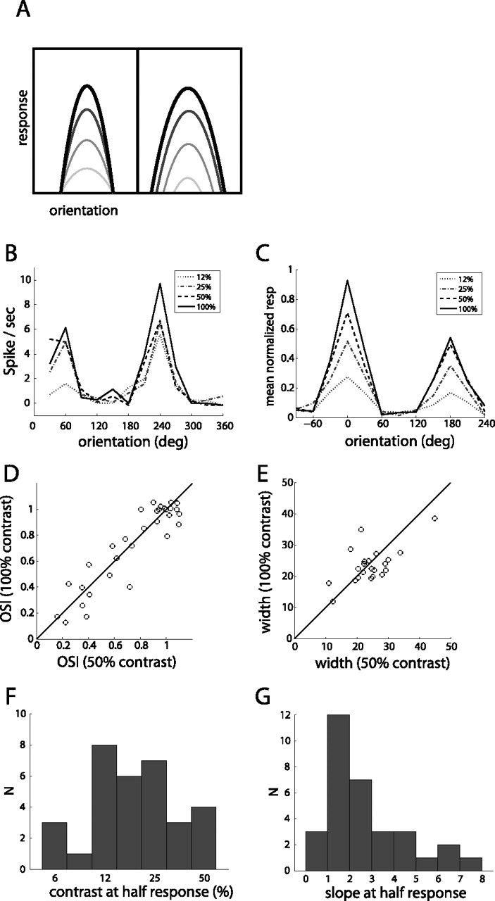
Contrast-invariant tuning and contrast–response characteristics. A, Schematic of contrast-invariant (left) versus contrast-dependent (right) orientation tuning. B, Example of orientation tuning in response to gratings of different contrast, for unit in Figure 2. C, Orientation tuning at different contrasts averaged across 22 orientation-selective units. Tuning curves of each unit were aligned to preferred orientation and normalized to maximum response before averaging. D, Comparison of orientation selectivity at 50 and 100% contrast shows no systematic change (n = 32). E, Width of tuning, for orientation-selective units (n = 22), at 50 and 100% contrast. F, Value of contrast that gave half-maximal response (n = 32). G, Slope of the contrast response function at half-maximal response.
We sought to determine whether this constancy is present in the mouse as well, to both assess the similarity in cortical processing to other species and ascertain whether genetic manipulations in mice could provide causal tests of proposed mechanisms of invariant tuning. For a subset of recordings (n = 6 animals), we presented drifting gratings of varying contrast and orientation, at fixed spatial frequency (0.04 cpd). A typical response from an oriented unit shown is shown in Figure 12 B, demonstrating contrast-invariant tuning, as the tuning curve only changes in amplitude, not shape, as contrast increases. Aligning and averaging the tuning curves of all orientation-selective units that responded to this spatial frequency (n = 22 units) resulted in the mean tuning curve observed in Figure 12 C, which shows no increase in width with increased contrast. Furthermore, a comparison of all individual orientation tuning curves at two different contrasts shows no systematic change in either orientation selectivity (Fig. 12 D) or tuning width (Fig. 12 E).
In addition to testing contrast-invariant tuning, this stimulus set allowed us to measure the response as a function of contrast for those units that were responsive to this spatial frequency. Figure 12 F shows the value of contrast that resulted in half-maximal response, which showed a wide range, with a median value of 19.8%. The slope of response over contrast at the half-maximal response is shown in Figure 12 G; for normalized contrast–response curves, a slope of 1 indicates a relatively linear increase in response with contrast, whereas a greater slope indicates a sharp transition from low to high response at the midsaturation contrast. Although many units had slope near 1, again there was a wide range, with a median value of 2.4.
Discussion
Despite the poor visual acuity (Prusky et al., 2000) and relatively small region of cortex devoted to visual processing, we find that most neurons in mouse V1 respond to at least one type of visual stimulus. We have determined the relevant range of stimulus parameters, such as spatial and temporal frequency, and orientation selectivity, which are effective in driving the strongest responses. This broad characterization should benefit future studies by guiding the design of appropriate visual stimuli. For instance, knowledge of orientation and spatial frequency tuning width can help specify the resolution at which these parameters should be sampled to properly characterize all cells. These results should also facilitate the design of optimal stimuli for other functional recording techniques that lack the single-spike temporal resolution of electrophysiology, such as intrinsic signal (Kalatsky and Stryker, 2003) or calcium imaging (Stosiek et al., 2003). Importantly, our finding that responses vary greatly across the layers indicates that there can be widely different results for simple measurements, such as the degree of orientation selectivity or receptive field size, depending on the distribution of recording sites in a given study.
Technical considerations
Several technical differences from previous experiments may contribute to the responsiveness and selectivity we observed. In terms of surgery, performing a small craniotomy and inserting the electrode at an angle to the cortical surface, which may reduce damage to superficial recording sites, aided in isolating units and evoking strong responses from the superficial layers, in which the most selective cells were found. In contrast to traditional single-electrode recording, which involves advancing an electrode until a responding unit is found, we allowed our multisite electrode to settle at one position and recorded any units that could be detected over 1 h or more of recording time. This enabled us to isolate units with low spontaneous rates and sparse responses. Indeed, some units were isolated that produced only a few hundred spikes over 1 h of recording. Traditional recording techniques that search for responses are most likely to detect units with high firing rates or large extracellular action potentials, which in mice tend to be the less selective layer 5 and putative inhibitory units. Furthermore, because isolated units were generally stable over this period, we were able to present a large number of stimuli, sampling a broad parameter space, to evoke responses from units with either very selective or poor responses.
We verified laminar identity using the LFP from geometrically defined recording sites established by the silicon probes, confirmed in several cases by retrospective histology. Although the layers in mouse cortex are not as clearly defined as in other species, with less distinct cytoarchitectural boundaries and a more extensive thalamic projection (Frost and Caviness, 1980; Antonini et al., 1999), we found clear differences in response types between these laminas.
Furthermore, spike waveforms were used to segregate units into narrow-spiking and broad-spiking categories, which have been used frequently as a rough classification of inhibitory versus excitatory neurons (Rao et al., 1999; Bruno and Simons, 2002; Andermann et al., 2004; Mitchell et al., 2007). There is still some uncertainty as to the exact cell types represented by this division, in particular whether the narrow-spiking class includes just the parvalbumin-positive fast-spiking units and whether some small fraction of narrow-spiking units may be excitatory (Swadlow, 2003). However, the profound difference in functional responses we find between these groups suggests that, although their exact categorization may be uncertain, narrow-spiking neurons are primarily a distinct class from broad-spiking neurons. Our designation of narrow-spiking units as putative inhibitory neurons is further supported by the recent finding, using two-photon calcium imaging in mouse, that inhibitory GABAergic neurons are much less orientation selective than non-GABAergic neurons (Sohya et al., 2007). It will be interesting to see whether such a dichotomy in orientation selectivity exists in other species that have a significant number of nonoriented units. Two recent studies in cat, in which almost all units are orientation selective, did show decreased orientation selectivity among presumed inhibitory neurons in layer 4 (Cardin et al., 2007; Nowak et al., 2008).
Comparison with previous studies
Our results generally agree with previous studies in mice, particularly the finding of greater orientation selectivity in superficial layers (Mangini and Pearlman, 1980; Metin et al., 1988), and the large number of poorly orientation-selective units with large receptive fields in layer 5, which have been suggested previously to be corticotectal neurons (Mangini and Pearlman, 1980). Our findings are also in agreement with recent studies in other rodents such as rat (Girman et al., 1999; Ohki et al., 2005) and squirrel (Van Hooser et al., 2005), confirming that high orientation selectivity can exist in the absence of large-scale organization such as an orientation map. We did not observe many of the simple, nonoriented responses in layer 4 that have been described in previous mouse studies (Mangini and Pearlman, 1980; Metin et al., 1988). It is likely that previous recordings with sharp tungsten electrodes more readily isolated afferents of LGN neurons, which generally have linear nonoriented responses. It is also possible that sinusoidal gratings elicit greater selectivity than small spots or flashed stimuli, used in some previous studies.
Our results are also consistent with previous finding in the mouse dorsal lateral geniculate nucleus (dLGN) of thalamus, which provides direct input to V1. Grubb and Thompson (2003) found a median peak spatial frequency response of 0.027 cpd, similar to our finding of 0.035 cpd. Our measurement of peak temporal frequency of 1.7 Hz, obtained with contrast-reversing rather than drifting gratings, shows a decrease from 3.8 Hz measured in dLGN, similar to the decrease in temporal frequency response from thalamus to cortex found in other species (Hawken et al., 1996). We do find slightly higher temporal frequency tuning in layer 4, consistent with its receiving direct input from thalamus.
It is also interesting to compare these findings in mouse with those of “higher” species whose visual systems have been more thoroughly studied (for an extensive comparison of tuning properties across species, see Van Hooser, 2007). The most readily apparent difference is in spatial scale, with median spatial frequency in mouse of 0.04 cpd compared with 0.9 cpd in cat and up to 4 cpd in primates. The total percentage of oriented units (74% of responsive units) is slightly lower, with many other species having 80% or more, although >95% of units in cat are reported to be orientation selective (Van Hooser, 2007). Within the population of oriented units, the width of tuning was close to that of other model species, with median orientation tuning half-width of 28–29° for mouse compared with 19–25° in cat and 24° in macaque (Van Hooser, 2007). The spatial frequency bandwidth of 2.5 octaves in mouse is somewhat larger than the value of 1.5 octaves in cat and macaque but close to owl monkey, 2.1 octaves, and squirrel, 2.3 octaves (Van Hooser, 2007). Thus, even at the low-resolution limit of the mouse visual system, neurons can still be nearly as selective for orientation and spatial frequency as in species with more developed visual systems. As pointed out previously (Van Hooser, 2007), these tuning widths seem to be fairly invariant across species and may represent common constraints on cortical processing.
One striking difference in mice is the relative paucity of complex cells in layer 2/3, in which we found that 75% of responsive units were simple, whereas in other species the majority of units outside of layer 4 are complex (Van Hooser, 2007). It is interesting to speculate that this may be related to the absence of orientation columns in mouse. Most models of complex responses involve pooling inputs of similar orientation, which can result from nearest-neighbor connectivity in the presence of orientation columns. However, without columnar anatomical organization, greater constraints on synaptic specificity would be needed to preserve orientation selectivity while pooling inputs. It must be noted, however, that the squirrel has a large proportion of complex cells but lacks an orientation map (Van Hooser et al., 2005).
The relative lack of orientation and phase selectivity in putative inhibitory neurons has interesting implications for cortical processing. They would be well situated to provide signals such as divisive normalization (Carandini et al., 1997), balanced inhibition and excitation (Chance et al., 2002), untuned inhibition for contrast-invariant tuning (Lauritzen and Miller, 2003), and for coupling net activity to metabolism or blood flow (Buzsáki et al., 2007). Conversely, many models of orientation selectivity require orientation-selective inhibition (Ferster and Miller, 2000), and the net inhibitory input to cat cortical cells has in fact been shown to be orientation tuned (Anderson et al., 2000). Only a small fraction of putative inhibitory units we recorded have sufficient orientation selectivity to provide such a signal. It is possible that this fraction of oriented narrow-spiking units, or perhaps inhibitory neurons among the broad-spiking units, serves this distinct role; alternatively tuned inhibition may not be necessary for contrast-invariant orientation selectivity (Finn et al., 2007; Priebe and Ferster, 2008).
Future directions
The presence of strong selectivity and differential responses by layer and cell type opens the door for additional study of cortical development and function, taking advantage of recent technical advances using mouse genetics to study neural circuitry. For example, viral-based labels for synaptic connectivity (Wickersham et al., 2007) could be used to investigate the relative tuning properties of connected neurons and, in combination with cell-type specific markers, could elucidate the microcircuit that gives rise to selective responses. The use of quantitative visual analysis with manipulations of genes involved in growth and synaptic plasticity may elucidate the developmental processes that result in specific receptive field properties, such as organized ON and OFF subregions resulting in orientation selectivity and simple versus complex cell types. Finally, the ability to make precise manipulations of neural activity in defined cell populations (Boyden et al., 2005; Tan et al., 2006; Zhang et al., 2007b) should allow direct causal tests of models of cortical processing.
Footnotes
This work was supported by National Institutes of Health Grant EY02874 (M.P.S.) and a Helen Hay Whitney Foundation fellowship (C.M.N.). We thank Drs. Jonathan Horton, Steve Lisberger, and Linda Wilbrecht and members of the Stryker laboratory for comments on this manuscript and helpful discussions. We also thank Drs. Michael Lewicki and Eizaburo Doi for providing routines to fit Gabor functions and Dr. Dario Ringach for data on Gabor fits and circular variance from macaque.
References
- Andermann et al., 2004.Andermann ML, Ritt J, Neimark MA, Moore CI. Neural correlates of vibrissa resonance; band-pass and somatotopic representation of high-frequency stimuli. Neuron. 2004;42:451–463. doi: 10.1016/s0896-6273(04)00198-9. [DOI] [PubMed] [Google Scholar]
- Anderson et al., 2000.Anderson JS, Carandini M, Ferster D. Orientation tuning of input conductance, excitation, and inhibition in cat primary visual cortex. J Neurophysiol. 2000;84:909–926. doi: 10.1152/jn.2000.84.2.909. [DOI] [PubMed] [Google Scholar]
- Antonini et al., 1999.Antonini A, Fagiolini M, Stryker MP. Anatomical correlates of functional plasticity in mouse visual cortex. J Neurosci. 1999;19:4388–4406. doi: 10.1523/JNEUROSCI.19-11-04388.1999. [DOI] [PMC free article] [PubMed] [Google Scholar]
- Atencio and Schreiner, 2008.Atencio CA, Schreiner CE. Spectrotemporal processing differences between auditory cortical fast-spiking and regular-spiking neurons. J Neurosci. 2008;28:3897–3910. doi: 10.1523/JNEUROSCI.5366-07.2008. [DOI] [PMC free article] [PubMed] [Google Scholar]
- Barthó et al., 2004.Barthó P, Hirase H, Monconduit L, Zugaro M, Harris KD, Buzsáki G. Characterization of neocortical principal cells and interneurons by network interactions and extracellular features. J Neurophysiol. 2004;92:600–608. doi: 10.1152/jn.01170.2003. [DOI] [PubMed] [Google Scholar]
- Boyden et al., 2005.Boyden ES, Zhang F, Bamberg E, Nagel G, Deisseroth K. Millisecond-timescale, genetically targeted optical control of neural activity. Nat Neurosci. 2005;8:1263–1268. doi: 10.1038/nn1525. [DOI] [PubMed] [Google Scholar]
- Brainard, 1997.Brainard DH. The psychophysics toolbox. Spat Vis. 1997;10:433–436. [PubMed] [Google Scholar]
- Brecht et al., 2003.Brecht M, Roth A, Sakmann B. Dynamic receptive fields of reconstructed pyramidal cells in layers 3 and 2 of rat somatosensory barrel cortex. J Physiol (Lond) 2003;553:243–265. doi: 10.1113/jphysiol.2003.044222. [DOI] [PMC free article] [PubMed] [Google Scholar]
- Brecht et al., 2004.Brecht M, Fee MS, Garaschuk O, Helmchen F, Margrie TW, Svoboda K, Osten P. Novel approaches to monitor and manipulate single neurons in vivo . J Neurosci. 2004;24:9223–9227. doi: 10.1523/JNEUROSCI.3344-04.2004. [DOI] [PMC free article] [PubMed] [Google Scholar]
- Bruno and Simons, 2002.Bruno RM, Simons DJ. Feedforward mechanisms of excitatory and inhibitory cortical receptive fields. J Neurosci. 2002;22:10966–10975. doi: 10.1523/JNEUROSCI.22-24-10966.2002. [DOI] [PMC free article] [PubMed] [Google Scholar]
- Buzsáki and Draguhn, 2004.Buzsáki G, Draguhn A. Neuronal oscillations in cortical networks. Science. 2004;304:1926–1929. doi: 10.1126/science.1099745. [DOI] [PubMed] [Google Scholar]
- Buzsáki et al., 2007.Buzsáki G, Kaila K, Raichle M. Inhibition and brain work. Neuron. 2007;56:771–783. doi: 10.1016/j.neuron.2007.11.008. [DOI] [PMC free article] [PubMed] [Google Scholar]
- Callaway, 2005.Callaway EM. A molecular and genetic arsenal for systems neuroscience. Trends Neurosci. 2005;28:196–201. doi: 10.1016/j.tins.2005.01.007. [DOI] [PubMed] [Google Scholar]
- Cang et al., 2005.Cang J, Kaneko M, Yamada J, Woods G, Stryker MP, Feldheim DA. Ephrin-as guide the formation of functional maps in the visual cortex. Neuron. 2005;48:577–589. doi: 10.1016/j.neuron.2005.10.026. [DOI] [PMC free article] [PubMed] [Google Scholar]
- Carandini et al., 1997.Carandini M, Heeger DJ, Movshon JA. Linearity and normalization in simple cells of the macaque primary visual cortex. J Neurosci. 1997;17:8621–8644. doi: 10.1523/JNEUROSCI.17-21-08621.1997. [DOI] [PMC free article] [PubMed] [Google Scholar]
- Carandini et al., 2005.Carandini M, Demb JB, Mante V, Tolhurst DJ, Dan Y, Olshausen BA, Gallant JL, Rust NC. Do we know what the early visual system does? J Neurosci. 2005;25:10577–10597. doi: 10.1523/JNEUROSCI.3726-05.2005. [DOI] [PMC free article] [PubMed] [Google Scholar]
- Cardin et al., 2007.Cardin JA, Palmer LA, Contreras D. Stimulus feature selectivity in excitatory and inhibitory neurons in primary visual cortex. J Neurosci. 2007;27:10333–10344. doi: 10.1523/JNEUROSCI.1692-07.2007. [DOI] [PMC free article] [PubMed] [Google Scholar]
- Chance et al., 2002.Chance FS, Abbott LF, Reyes AD. Gain modulation from background synaptic input. Neuron. 2002;35:773–782. doi: 10.1016/s0896-6273(02)00820-6. [DOI] [PubMed] [Google Scholar]
- Chichilnisky, 2001.Chichilnisky EJ. A simple white noise analysis of neuronal light responses. Network. 2001;12:199–213. [PubMed] [Google Scholar]
- Connors and Kriegstein, 1986.Connors BW, Kriegstein AR. Cellular physiology of the turtle visual cortex: distinctive properties of pyramidal and stellate neurons. J Neurosci. 1986;6:164–177. doi: 10.1523/JNEUROSCI.06-01-00164.1986. [DOI] [PMC free article] [PubMed] [Google Scholar]
- DeAngelis et al., 1993.DeAngelis GC, Ohzawa I, Freeman RD. Spatiotemporal organization of simple-cell receptive fields in the cat's striate cortex. I. General characteristics and postnatal development. J Neurophysiol. 1993;69:1091–1117. doi: 10.1152/jn.1993.69.4.1091. [DOI] [PubMed] [Google Scholar]
- DeWeese et al., 2003.DeWeese MR, Wehr M, Zador AM. Binary spiking in auditory cortex. J Neurosci. 2003;23:7940–7949. doi: 10.1523/JNEUROSCI.23-21-07940.2003. [DOI] [PMC free article] [PubMed] [Google Scholar]
- Douglas and Martin, 2004.Douglas RJ, Martin KA. Neuronal circuits of the neocortex. Annu Rev Neurosci. 2004;27:419–451. doi: 10.1146/annurev.neuro.27.070203.144152. [DOI] [PubMed] [Google Scholar]
- Dräger, 1975.Dräger UC. Receptive fields of single cells and topography in mouse visual cortex. J Comp Neurol. 1975;160:269–290. doi: 10.1002/cne.901600302. [DOI] [PubMed] [Google Scholar]
- Fagiolini et al., 1994.Fagiolini M, Pizzorusso T, Berardi N, Domenici L, Maffei L. Functional postnatal development of the rat primary visual cortex and the role of visual experience: dark rearing and monocular deprivation. Vision Res. 1994;34:709–720. doi: 10.1016/0042-6989(94)90210-0. [DOI] [PubMed] [Google Scholar]
- Fagiolini et al., 2003.Fagiolini M, Katagiri H, Miyamoto H, Mori H, Grant SG, Mishina M, Hensch TK. Separable features of visual cortical plasticity revealed by N-methyl-d-aspartate receptor 2A signaling. Proc Natl Acad Sci USA. 2003;100:2854–2859. doi: 10.1073/pnas.0536089100. [DOI] [PMC free article] [PubMed] [Google Scholar]
- Fagiolini et al., 2004.Fagiolini M, Fritschy JM, Löw K, Möhler H, Rudolph U, Hensch TK. Specific GABAA circuits for visual cortical plasticity. Science. 2004;303:1681–1683. doi: 10.1126/science.1091032. [DOI] [PubMed] [Google Scholar]
- Feng et al., 2000.Feng G, Mellor RH, Bernstein M, Keller-Peck C, Nguyen QT, Wallace M, Nerbonne JM, Lichtman JW, Sanes JR. Imaging neuronal subsets in transgenic mice expressing multiple spectral variants of GFP. Neuron. 2000;28:41–51. doi: 10.1016/s0896-6273(00)00084-2. [DOI] [PubMed] [Google Scholar]
- Ferster and Miller, 2000.Ferster D, Miller KD. Neural mechanisms of orientation selectivity in the visual cortex. Annu Rev Neurosci. 2000;23:441–471. doi: 10.1146/annurev.neuro.23.1.441. [DOI] [PubMed] [Google Scholar]
- Field and Tolhurst, 1986.Field DJ, Tolhurst DJ. The structure and symmetry of simple-cell receptive-field profiles in the cat's visual cortex. Proc R Soc Lond B Biol Sci. 1986;228:379–400. doi: 10.1098/rspb.1986.0060. [DOI] [PubMed] [Google Scholar]
- Finn et al., 2007.Finn IM, Priebe NJ, Ferster D. The emergence of contrast-invariant orientation tuning in simple cells of cat visual cortex. Neuron. 2007;54:137–152. doi: 10.1016/j.neuron.2007.02.029. [DOI] [PMC free article] [PubMed] [Google Scholar]
- Frost and Caviness, 1980.Frost DO, Caviness VS., Jr Radial organization of thalamic projections to the neocortex in the mouse. J Comp Neurol. 1980;194:369–393. doi: 10.1002/cne.901940206. [DOI] [PubMed] [Google Scholar]
- Gilbert, 1983.Gilbert CD. Microcircuitry of the visual cortex. Annu Rev Neurosci. 1983;6:217–247. doi: 10.1146/annurev.ne.06.030183.001245. [DOI] [PubMed] [Google Scholar]
- Girman et al., 1999.Girman SV, Sauvé Y, Lund RD. Receptive field properties of single neurons in rat primary visual cortex. J Neurophysiol. 1999;82:301–311. doi: 10.1152/jn.1999.82.1.301. [DOI] [PubMed] [Google Scholar]
- Grubb and Thompson, 2003.Grubb MS, Thompson ID. Quantitative characterization of visual response properties in the mouse dorsal lateral geniculate nucleus. J Neurophysiol. 2003;90:3594–3607. doi: 10.1152/jn.00699.2003. [DOI] [PubMed] [Google Scholar]
- Harris et al., 2000.Harris KD, Henze DA, Csicsvari J, Hirase H, Buzsáki G. Accuracy of tetrode spike separation as determined by simultaneous intracellular and extracellular measurements. J Neurophysiol. 2000;84:401–414. doi: 10.1152/jn.2000.84.1.401. [DOI] [PubMed] [Google Scholar]
- Hasenstaub et al., 2005.Hasenstaub A, Shu Y, Haider B, Kraushaar U, Duque A, McCormick DA. Inhibitory postsynaptic potentials carry synchronized frequency information in active cortical networks. Neuron. 2005;47:423–435. doi: 10.1016/j.neuron.2005.06.016. [DOI] [PubMed] [Google Scholar]
- Hawken and Parker, 1987.Hawken MJ, Parker AJ. Spatial properties of neurons in the monkey striate cortex. Proc R Soc Lond B Biol Sci. 1987;231:251–288. doi: 10.1098/rspb.1987.0044. [DOI] [PubMed] [Google Scholar]
- Hawken et al., 1996.Hawken MJ, Shapley RM, Grosof DH. Temporal-frequency selectivity in monkey visual cortex. Vis Neurosci. 1996;13:477–492. doi: 10.1017/s0952523800008154. [DOI] [PubMed] [Google Scholar]
- Heimel et al., 2005.Heimel JA, Van Hooser SD, Nelson SB. Laminar organization of response properties in primary visual cortex of the gray squirrel (Sciurus carolinensis) J Neurophysiol. 2005;94:3538–3554. doi: 10.1152/jn.00106.2005. [DOI] [PubMed] [Google Scholar]
- Hensch, 2005.Hensch TK. Critical period plasticity in local cortical circuits. Nat Rev Neurosci. 2005;6:877–888. doi: 10.1038/nrn1787. [DOI] [PubMed] [Google Scholar]
- Hofer et al., 2006.Hofer SB, Mrsic-Flogel TD, Bonhoeffer T, Hübener M. Lifelong learning: ocular dominance plasticity in mouse visual cortex. Curr Opin Neurobiol. 2006;16:451–459. doi: 10.1016/j.conb.2006.06.007. [DOI] [PubMed] [Google Scholar]
- Huang et al., 1999.Huang ZJ, Kirkwood A, Pizzorusso T, Porciatti V, Morales B, Bear MF, Maffei L, Tonegawa S. BDNF regulates the maturation of inhibition and the critical period of plasticity in mouse visual cortex. Cell. 1999;98:739–755. doi: 10.1016/s0092-8674(00)81509-3. [DOI] [PubMed] [Google Scholar]
- Hubel and Wiesel, 1962.Hubel DH, Wiesel TN. Receptive fields, binocular interaction and functional architecture in the cat's visual cortex. J Physiol (Lond) 1962;160:106–154. doi: 10.1113/jphysiol.1962.sp006837. [DOI] [PMC free article] [PubMed] [Google Scholar]
- Hübener, 2003.Hübener M. Mouse visual cortex. Curr Opin Neurobiol. 2003;13:413–420. doi: 10.1016/s0959-4388(03)00102-8. [DOI] [PubMed] [Google Scholar]
- Issa et al., 2000.Issa NP, Trepel C, Stryker MP. Spatial frequency maps in cat visual cortex. J Neurosci. 2000;20:8504–8514. doi: 10.1523/JNEUROSCI.20-22-08504.2000. [DOI] [PMC free article] [PubMed] [Google Scholar]
- Jeon et al., 1998.Jeon CJ, Strettoi E, Masland RH. The major cell populations of the mouse retina. J Neurosci. 1998;18:8936–8946. doi: 10.1523/JNEUROSCI.18-21-08936.1998. [DOI] [PMC free article] [PubMed] [Google Scholar]
- Jones and Palmer, 1987a.Jones JP, Palmer LA. The two-dimensional spatial structure of simple receptive fields in cat striate cortex. J Neurophysiol. 1987a;58:1187–1211. doi: 10.1152/jn.1987.58.6.1187. [DOI] [PubMed] [Google Scholar]
- Jones and Palmer, 1987b.Jones JP, Palmer LA. An evaluation of the two-dimensional Gabor filter model of simple receptive fields in cat striate cortex. J Neurophysiol. 1987b;58:1233–1258. doi: 10.1152/jn.1987.58.6.1233. [DOI] [PubMed] [Google Scholar]
- Kalatsky and Stryker, 2003.Kalatsky VA, Stryker MP. New paradigm for optical imaging: temporally encoded maps of intrinsic signal. Neuron. 2003;38:529–545. doi: 10.1016/s0896-6273(03)00286-1. [DOI] [PubMed] [Google Scholar]
- Karpova et al., 2005.Karpova AY, Tervo DG, Gray NW, Svoboda K. Rapid and reversible chemical inactivation of synaptic transmission in genetically targeted neurons. Neuron. 2005;48:727–735. doi: 10.1016/j.neuron.2005.11.015. [DOI] [PubMed] [Google Scholar]
- Lauritzen and Miller, 2003.Lauritzen TZ, Miller KD. Different roles for simple-cell and complex-cell inhibition in V1. J Neurosci. 2003;23:10201–10213. doi: 10.1523/JNEUROSCI.23-32-10201.2003. [DOI] [PMC free article] [PubMed] [Google Scholar]
- Lee et al., 2007.Lee SH, Land PW, Simons DJ. Layer- and cell-type-specific effects of neonatal whisker-trimming in adult rat barrel cortex. J Neurophysiol. 2007;97:4380–4385. doi: 10.1152/jn.01217.2006. [DOI] [PubMed] [Google Scholar]
- Mangini and Pearlman, 1980.Mangini NJ, Pearlman AL. Laminar distribution of receptive field properties in the primary visual cortex of the mouse. J Comp Neurol. 1980;193:203–222. doi: 10.1002/cne.901930114. [DOI] [PubMed] [Google Scholar]
- McCormick et al., 1985.McCormick DA, Connors BW, Lighthall JW, Prince DA. Comparative electrophysiology of pyramidal and sparsely spiny stellate neurons of the neocortex. J Neurophysiol. 1985;54:782–806. doi: 10.1152/jn.1985.54.4.782. [DOI] [PubMed] [Google Scholar]
- Mechler and Ringach, 2002.Mechler F, Ringach DL. On the classification of simple and complex cells. Vision Res. 2002;42:1017–1033. doi: 10.1016/s0042-6989(02)00025-1. [DOI] [PubMed] [Google Scholar]
- Métin et al., 1988.Métin C, Godement P, Imbert M. The primary visual cortex in the mouse: receptive field properties and functional organization. Exp Brain Res. 1988;69:594–612. doi: 10.1007/BF00247312. [DOI] [PubMed] [Google Scholar]
- Mitchell et al., 2007.Mitchell JF, Sundberg KA, Reynolds JH. Differential attention-dependent response modulation across cell classes in macaque visual area V4. Neuron. 2007;55:131–141. doi: 10.1016/j.neuron.2007.06.018. [DOI] [PubMed] [Google Scholar]
- Mitzdorf, 1985.Mitzdorf U. Current source-density method and application in cat cerebral cortex: investigation of evoked potentials and EEG phenomena. Physiol Rev. 1985;65:37–100. doi: 10.1152/physrev.1985.65.1.37. [DOI] [PubMed] [Google Scholar]
- Naka and Rushton, 1966.Naka KI, Rushton WA. S-potentials from colour units in the retina of fish (Cyprinidae) J Physiol (Lond) 1966;185:536–555. doi: 10.1113/jphysiol.1966.sp008001. [DOI] [PMC free article] [PubMed] [Google Scholar]
- Nase et al., 2003.Nase G, Singer W, Monyer H, Engel AK. Features of neuronal synchrony in mouse visual cortex. J Neurophysiol. 2003;90:1115–1123. doi: 10.1152/jn.00480.2002. [DOI] [PubMed] [Google Scholar]
- Nowak et al., 2008.Nowak LG, Sanchez-Vives MV, McCormick DA. Lack of orientation and direction selectivity in a subgroup of fast-spiking inhibitory interneurons: cellular and synaptic mechanisms and comparison with other electrophysiological cell types. Cereb Cortex. 2008;18:1058–1078. doi: 10.1093/cercor/bhm137. [DOI] [PMC free article] [PubMed] [Google Scholar]
- Ohki and Reid, 2007.Ohki K, Reid RC. Specificity and randomness in the visual cortex. Curr Opin Neurobiol. 2007;17:401–407. doi: 10.1016/j.conb.2007.07.007. [DOI] [PMC free article] [PubMed] [Google Scholar]
- Ohki et al., 2005.Ohki K, Chung S, Ch'ng YH, Kara P, Reid RC. Functional imaging with cellular resolution reveals precise micro-architecture in visual cortex. Nature. 2005;433:597–603. doi: 10.1038/nature03274. [DOI] [PubMed] [Google Scholar]
- Pelli, 1997.Pelli DG. The VideoToolbox software for visual psychophysics: transforming numbers into movies. Spat Vis. 1997;10:437–442. [PubMed] [Google Scholar]
- Polleux et al., 2007.Polleux F, Ince-Dunn G, Ghosh A. Transcriptional regulation of vertebrate axon guidance and synapse formation. Nat Rev Neurosci. 2007;8:331–340. doi: 10.1038/nrn2118. [DOI] [PubMed] [Google Scholar]
- Priebe and Ferster, 2008.Priebe NJ, Ferster D. Inhibition, spike threshold, and stimulus selectivity in primary visual cortex. Neuron. 2008;57:482–497. doi: 10.1016/j.neuron.2008.02.005. [DOI] [PubMed] [Google Scholar]
- Prusky et al., 2000.Prusky GT, West PW, Douglas RM. Behavioral assessment of visual acuity in mice and rats. Vision Res. 2000;40:2201–2209. doi: 10.1016/s0042-6989(00)00081-x. [DOI] [PubMed] [Google Scholar]
- Rao et al., 1999.Rao SG, Williams GV, Goldman-Rakic PS. Isodirectional tuning of adjacent interneurons and pyramidal cells during working memory: evidence for microcolumnar organization in PFC. J Neurophysiol. 1999;81:1903–1916. doi: 10.1152/jn.1999.81.4.1903. [DOI] [PubMed] [Google Scholar]
- Rash and Grove, 2006.Rash BG, Grove EA. Area and layer patterning in the developing cerebral cortex. Curr Opin Neurobiol. 2006;16:25–34. doi: 10.1016/j.conb.2006.01.004. [DOI] [PubMed] [Google Scholar]
- Ringach, 2002.Ringach DL. Spatial structure and symmetry of simple-cell receptive fields in macaque primary visual cortex. J Neurophysiol. 2002;88:455–463. doi: 10.1152/jn.2002.88.1.455. [DOI] [PubMed] [Google Scholar]
- Ringach, 2004.Ringach DL. Mapping receptive fields in primary visual cortex. J Physiol (Lond) 2004;558:717–728. doi: 10.1113/jphysiol.2004.065771. [DOI] [PMC free article] [PubMed] [Google Scholar]
- Ringach et al., 1997.Ringach DL, Sapiro G, Shapley R. A subspace reverse-correlation technique for the study of visual neurons. Vision Res. 1997;37:2455–2464. doi: 10.1016/s0042-6989(96)00247-7. [DOI] [PubMed] [Google Scholar]
- Ringach et al., 2002.Ringach DL, Shapley RM, Hawken MJ. Orientation selectivity in macaque V1: diversity and laminar dependence. J Neurosci. 2002;22:5639–5651. doi: 10.1523/JNEUROSCI.22-13-05639.2002. [DOI] [PMC free article] [PubMed] [Google Scholar]
- Sato et al., 2007.Sato TR, Gray NW, Mainen ZF, Svoboda K. The functional microarchitecture of the mouse barrel cortex. PLoS Biol. 2007;5:e189. doi: 10.1371/journal.pbio.0050189. [DOI] [PMC free article] [PubMed] [Google Scholar]
- Sawtell et al., 2003.Sawtell NB, Frenkel MY, Philpot BD, Nakazawa K, Tonegawa S, Bear MF. NMDA receptor-dependent ocular dominance plasticity in adult visual cortex. Neuron. 2003;38:977–985. doi: 10.1016/s0896-6273(03)00323-4. [DOI] [PubMed] [Google Scholar]
- Schmitzer-Torbert et al., 2005.Schmitzer-Torbert N, Jackson J, Henze D, Harris K, Redish AD. Quantitative measures of cluster quality for use in extracellular recordings. Neuroscience. 2005;131:1–11. doi: 10.1016/j.neuroscience.2004.09.066. [DOI] [PubMed] [Google Scholar]
- Shapley et al., 2003.Shapley R, Hawken M, Ringach DL. Dynamics of orientation selectivity in the primary visual cortex and the importance of cortical inhibition. Neuron. 2003;38:689–699. doi: 10.1016/s0896-6273(03)00332-5. [DOI] [PubMed] [Google Scholar]
- Sharpee et al., 2004.Sharpee T, Rust NC, Bialek W. Analyzing neural responses to natural signals: maximally informative dimensions. Neural Comput. 2004;16:223–250. doi: 10.1162/089976604322742010. [DOI] [PubMed] [Google Scholar]
- Skottun et al., 1991.Skottun BC, De Valois RL, Grosof DH, Movshon JA, Albrecht DG, Bonds AB. Classifying simple and complex cells on the basis of response modulation. Vision Res. 1991;31:1079–1086. doi: 10.1016/0042-6989(91)90033-2. [DOI] [PubMed] [Google Scholar]
- Snellings et al., 2006.Snellings A, Anderson DJ, Aldridge JW. Improved signal and reduced noise in neural recordings from close-spaced electrode arrays using independent component analysis as a preprocessor. J Neurosci Methods. 2006;150:254–264. doi: 10.1016/j.jneumeth.2005.06.022. [DOI] [PubMed] [Google Scholar]
- Sohya et al., 2007.Sohya K, Kameyama K, Yanagawa Y, Obata K, Tsumoto T. GABAergic neurons are less selective to stimulus orientation than excitatory neurons in layer II/III of visual cortex, as revealed by in vivo functional Ca2+ imaging in transgenic mice. J Neurosci. 2007;27:2145–2149. doi: 10.1523/JNEUROSCI.4641-06.2007. [DOI] [PMC free article] [PubMed] [Google Scholar]
- Sompolinsky and Shapley, 1997.Sompolinsky H, Shapley R. New perspectives on the mechanisms for orientation selectivity. Curr Opin Neurobiol. 1997;7:514–522. doi: 10.1016/s0959-4388(97)80031-1. [DOI] [PubMed] [Google Scholar]
- Stosiek et al., 2003.Stosiek C, Garaschuk O, Holthoff K, Konnerth A. In vivo two-photon calcium imaging of neuronal networks. Proc Natl Acad Sci USA. 2003;100:7319–7324. doi: 10.1073/pnas.1232232100. [DOI] [PMC free article] [PubMed] [Google Scholar]
- Swadlow, 2003.Swadlow HA. Fast-spike interneurons and feedforward inhibition in awake sensory neocortex. Cereb Cortex. 2003;13:25–32. doi: 10.1093/cercor/13.1.25. [DOI] [PubMed] [Google Scholar]
- Swadlow et al., 2002.Swadlow HA, Gusev AG, Bezdudnaya T. Activation of a cortical column by a thalamocortical impulse. J Neurosci. 2002;22:7766–7773. doi: 10.1523/JNEUROSCI.22-17-07766.2002. [DOI] [PMC free article] [PubMed] [Google Scholar]
- Syken et al., 2006.Syken J, Grandpre T, Kanold PO, Shatz CJ. PirB restricts ocular-dominance plasticity in visual cortex. Science. 2006;313:1795–1800. doi: 10.1126/science.1128232. [DOI] [PubMed] [Google Scholar]
- Tamamaki et al., 2003.Tamamaki N, Yanagawa Y, Tomioka R, Miyazaki J, Obata K, Kaneko T. Green fluorescent protein expression and colocalization with calretinin, parvalbumin, and somatostatin in the GAD67-GFP knock-in mouse. J Comp Neurol. 2003;467:60–79. doi: 10.1002/cne.10905. [DOI] [PubMed] [Google Scholar]
- Tan et al., 2006.Tan EM, Yamaguchi Y, Horwitz GD, Gosgnach S, Lein ES, Goulding M, Albright TD, Callaway EM. Selective and quickly reversible inactivation of mammalian neurons in vivo using the Drosophila allatostatin receptor. Neuron. 2006;51:157–170. doi: 10.1016/j.neuron.2006.06.018. [DOI] [PubMed] [Google Scholar]
- Theunissen et al., 2001.Theunissen FE, David SV, Singh NC, Hsu A, Vinje WE, Gallant JL. Estimating spatio-temporal receptive fields of auditory and visual neurons from their responses to natural stimuli. Network. 2001;12:289–316. [PubMed] [Google Scholar]
- Van Hooser, 2007.Van Hooser SD. Similarity and diversity in visual cortex: is there a unifying theory of cortical computation? The Neuroscientist. 2007;13:639–656. doi: 10.1177/1073858407306597. [DOI] [PubMed] [Google Scholar]
- Van Hooser et al., 2005.Van Hooser SD, Heimel JA, Chung S, Nelson SB, Toth LJ. Orientation selectivity without orientation maps in visual cortex of a highly visual mammal. J Neurosci. 2005;25:19–28. doi: 10.1523/JNEUROSCI.4042-04.2005. [DOI] [PMC free article] [PubMed] [Google Scholar]
- Waites et al., 2005.Waites CL, Craig AM, Garner CC. Mechanisms of vertebrate synaptogenesis. Annu Rev Neurosci. 2005;28:251–274. doi: 10.1146/annurev.neuro.27.070203.144336. [DOI] [PubMed] [Google Scholar]
- Wickersham et al., 2007.Wickersham IR, Lyon DC, Barnard RJ, Mori T, Finke S, Conzelmann KK, Young JA, Callaway EM. Monosynaptic restriction of transsynaptic tracing from single, genetically targeted neurons. Neuron. 2007;53:639–647. doi: 10.1016/j.neuron.2007.01.033. [DOI] [PMC free article] [PubMed] [Google Scholar]
- Zeng et al., 2001.Zeng H, Chattarji S, Barbarosie M, Rondi-Reig L, Philpot BD, Miyakawa T, Bear MF, Tonegawa S. Forebrain-specific calcineurin knockout selectively impairs bidirectional synaptic plasticity and working/episodic-like memory. Cell. 2001;107:617–629. doi: 10.1016/s0092-8674(01)00585-2. [DOI] [PubMed] [Google Scholar]
- Zhang et al., 2007a.Zhang F, Aravanis AM, Adamantidis A, de Lecea L, Deisseroth K. Circuit-breakers: optical technologies for probing neural signals and systems. Nat Rev Neurosci. 2007a;8:577–581. doi: 10.1038/nrn2192. [DOI] [PubMed] [Google Scholar]
- Zhang et al., 2007b.Zhang F, Wang LP, Brauner M, Liewald JF, Kay K, Watzke N, Wood PG, Bamberg E, Nagel G, Gottschalk A, Deisseroth K. Multimodal fast optical interrogation of neural circuitry. Nature. 2007b;446:633–639. doi: 10.1038/nature05744. [DOI] [PubMed] [Google Scholar]