Abstract
In interphase, the human genome sequence folds in three dimensions into a rich variety of locus-specific contact patterns. Cohesin and CTCF are key regulators; perturbing the levels of either greatly disrupts genome-wide folding as assayed by chromosome conformation capture methods. Still, how a given DNA sequence encodes a particular locus-specific folding pattern remains unknown. Here we present a convolutional neural network, Akita, that accurately predicts genome folding from DNA sequence alone. Representations learned by Akita underscore the importance of an orientation-specific grammar for CTCF binding sites. Akita learns predictive nucleotide-level features of genome folding, revealing impacts of nucleotides beyond the core CTCF motif. Once trained, Akita enables rapid in silico predictions. Leveraging this, we demonstrate how Akita can be used to perform in silico saturation mutagenesis, interpret eQTLs, make predictions for structural variants, and probe species-specific genome folding. Collectively, these results enable decoding genome function from sequence through structure.
Introduction
Recent research has advanced our understanding of the proteins driving and the sequences underpinning 3D genome folding in mammalian interphase, including the interplay between CTCF and cohesin1 and their roles in development and disease2. CTCF is an 11 zinc finger protein that binds specific DNA sequence motifs and impacts genome folding in an orientation-dependent fashion1, consistent with orientation-dependent halting of loop extrusion by cohesin3. Still, predicting the consequences of perturbing any individual CTCF site, or other regulatory element, on local genome folding remains a challenge. While disruptions of single bases can alter genome folding, in other cases genome folding is surprisingly resilient to large-scale deletions and structural variants4,5.
Previous modeling approaches for 3D genome folding fall in two broad categories: machine learning and polymer-based (Supplemental Note 1). Some approaches draw on features of both. The machine learning approaches are closer in spirit to ours but differ in several key ways. Specifically, prior applications of machine learning to the 3D genome have either: (1) relied on epigenomic information as inputs 6-9, which does not readily allow for predicting effects of DNA variants, or (2) predicted derived features of genome folding (e.g. peaks10,11), which depend heavily on minor algorithmic differences12. Making quantitative predictions from sequence poses a substantial challenge: base pair information must be propagated to megabase scales where locus-specific patterns become salient in chromosome contact maps.
Convolutional neural networks (CNNs) have emerged as powerful tools for modelling genomic data as a function of DNA sequence, directly learning DNA sequence features from the data. CNNs now make state-of-the-art predictions for transcription factor binding, DNA accessibility, transcription, and RNA-binding13-16. DNA sequence features learned by CNNs can be subsequently post-processed into interpretable forms17. Recently, the Basenji CNN was used to process very long sequences (~131kb) and learn distal regulatory element influences18, suggesting that genome folding could be tractable with CNNs.
Here we present Akita, a CNN to transform input DNA sequence into predicted locus-specific genome folding. Akita takes in ~1Mb (220 bp) of DNA sequence and predicts contact frequency maps for all pairs of ~2kb (2048bp) bins within this region. Crucially, this allows Akita to predict the effect of mutating single base pairs. Trained model and code are available at: https://github.com/calico/basenji/tree/master/manuscripts/akita.
Results
Akita: a convolutional neural network for predicting 3D genome folding
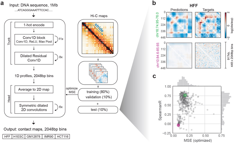
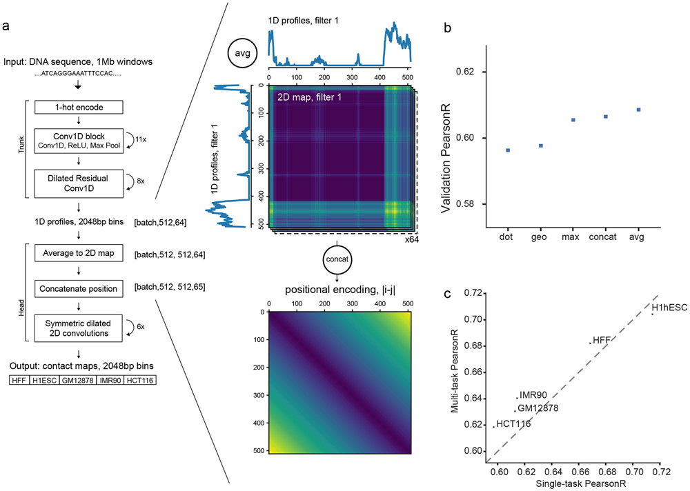
The Akita architecture consists of a ‘trunk’ based on the Basenji18,19 architecture to obtain 1D representations of genomic sequence, followed by a ‘head’ to transform to 2D maps of genome folding (Fig. 1a, Methods). In the ‘head’, we first averaged the representations of genomic bins i and j. Averaging produced slightly better generalization accuracy relative to several alternatives, including concatenation (Extended Data Fig. 1, Supplemental Note 2). As genomic distance can impact regulatory element communication, we appended a positional encoding of the distance between bins. Drawing inspiration from CNNs used in image processing, we computed multiple layers of dilated residual 2D convolutions, re-symmetrizing after each block. Finally, we compared the upper triangular regions of target and predicted maps. We reasoned that the trunk would enable Akita to learn DNA motifs and how they combine into a grammar for genome folding. In turn, the head would recognize relationships between these features and propagate this information across the map, while accounting for the dependencies between neighboring bins.
Figure 1: Akita, a convolutional neural network model for predicting 3D genome folding from DNA sequence.
a. Akita consists of a ‘trunk,’ based on the Basenji architecture18, followed by a ‘head’ to transform to 2D maps of genome folding. The trunk involves: (i) input 1Mb of 1-hot encoded DNA; (ii) 1D convolution blocks, where each block performs a max pool operation between adjacent positions to iteratively reduce to a bin size of 2048 bp; (iii) dilated residual 1D convolutions to propagate local information across the sequence. The ‘head’ involves: (i) forming 2D maps from the 1D vectors by averaging each pair of vectors at positions (i, j); (ii) symmetric dilated residual 2D convolutions; (iii) dense layer with linear activation to predict log(observed/expected) chromosome contact maps, with one separate output per dataset. We considered 2048bp binned maps, as high-quality Hi-C and Micro-C datasets ascertain genome folding at this resolution with tractable technical variance. We compared upper triangular regions of maps cropped by 32 bins on each side, making symmetric predictions for 448x448 bin (~917kb) maps. We trained our model on regions of the genome obtained by striding along Hi-C maps, using an 80/10/10 training/validation/test split.
b. Predicted and experimental log(observed/expected) contact frequency for two representative regions in the test set for Human Foreskin Fibroblast (HFF) Micro-C36. See Supplemental File 1 for images of predictions across the test set.
c. Quantification for the held-out test set: mean-squared error (MSE), which we optimize in model training, versus Spearman R, both calculated per region for each pair of targets and predictions for HFF Micro-C. Green and purple circles show regions from (b). Note correlations display a bimodal shape: regions with few locus-specific features have low MSE and low Spearman R.
We trained Akita with five of the highest-quality Hi-C and Micro-C datasets as targets (Methods, Table 1), first removing biases with genome-wide iterative correction (ICE20). We divided the genome into non-overlapping regions and used an 80/10/10 split to assign DNA sequences and their corresponding contact frequency map patches, megabase-by-megabase regions, to the training, validation, and test sets. As we aimed to predict locus-specific genome folding patterns, we normalized patches for distance-dependent decreases in contact frequency and took a log of their values to obtain the log(observed/expected) maps used as targets for Akita. We minimized the mean squared error (MSE) between predictions and targets, making a simultaneous prediction for each of the five datasets. We quantified model performance with MSE, as well as Pearson’s R and Spearman’s R of observed/expected maps on held-out ~1-Mb test set regions. The latter two correlation metrics are analogous to robust metrics for Hi-C map comparisons (e.g. HiCRep21).
Table 1:
Datasets used for training the human (hg38) model.
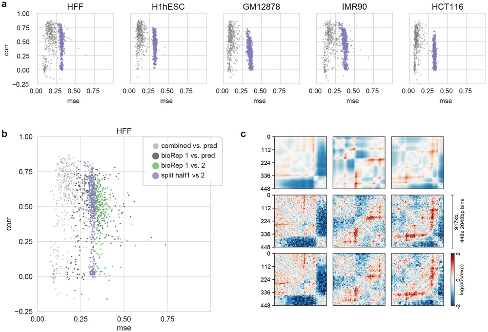
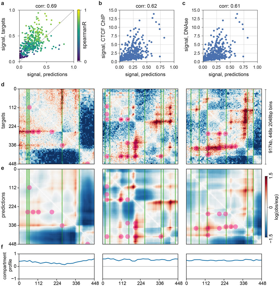
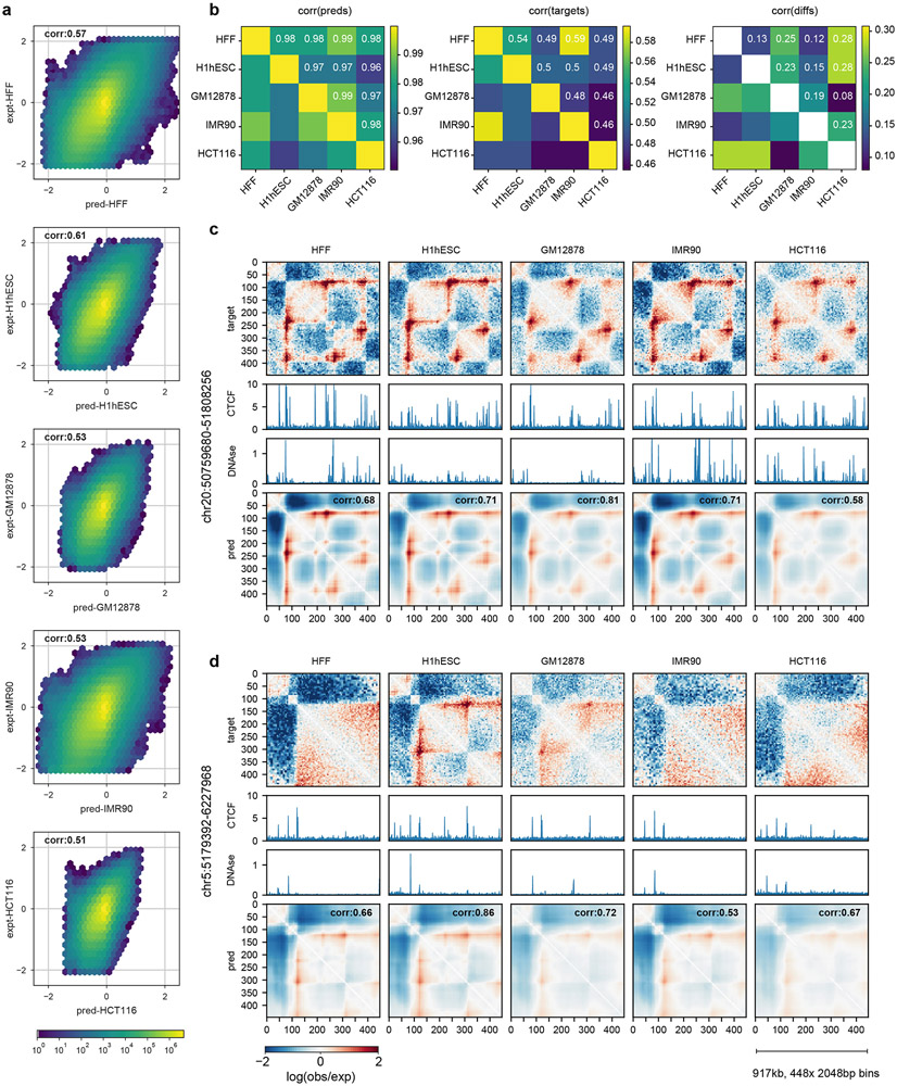
Akita learned a predictive representation of genome folding from DNA sequence, as evaluated on the held-out test set (genome-wide 0.14 MSE, 0.61 Pearson R, and 0.56 Spearman R). This performance approaches the limit set by noise between experimental replicates (Extended Data Fig. 2).On a region-by-region basis, Akita captured the variety of patterns seen experimentally (Fig. 1b,c). Individual maps with lower correlations often represented correct predictions for featureless experimental maps. Akita’s predictions reflected the strength of locus-specific folding seen experimentally (Extended Data Fig. 3a-c), and aligned well with Hi-C peaks and boundaries called in experimental data (Extended Data Fig. 3d-f). By simultaneously training on all five datasets in a multi-task framework, Akita achieved greater overall accuracy than models trained on single datasets alone (Extended Data Fig. 1c). Still, Akita predicted limited cell-type-specific differences (Extended Data Fig. 4). We hypothesize that this was constrained by the number of loci with strong cell-type-specific differences ascertainable in current experiments.
Akita learns accurate representations of genome folding from DNA sequence
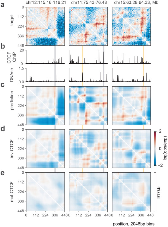
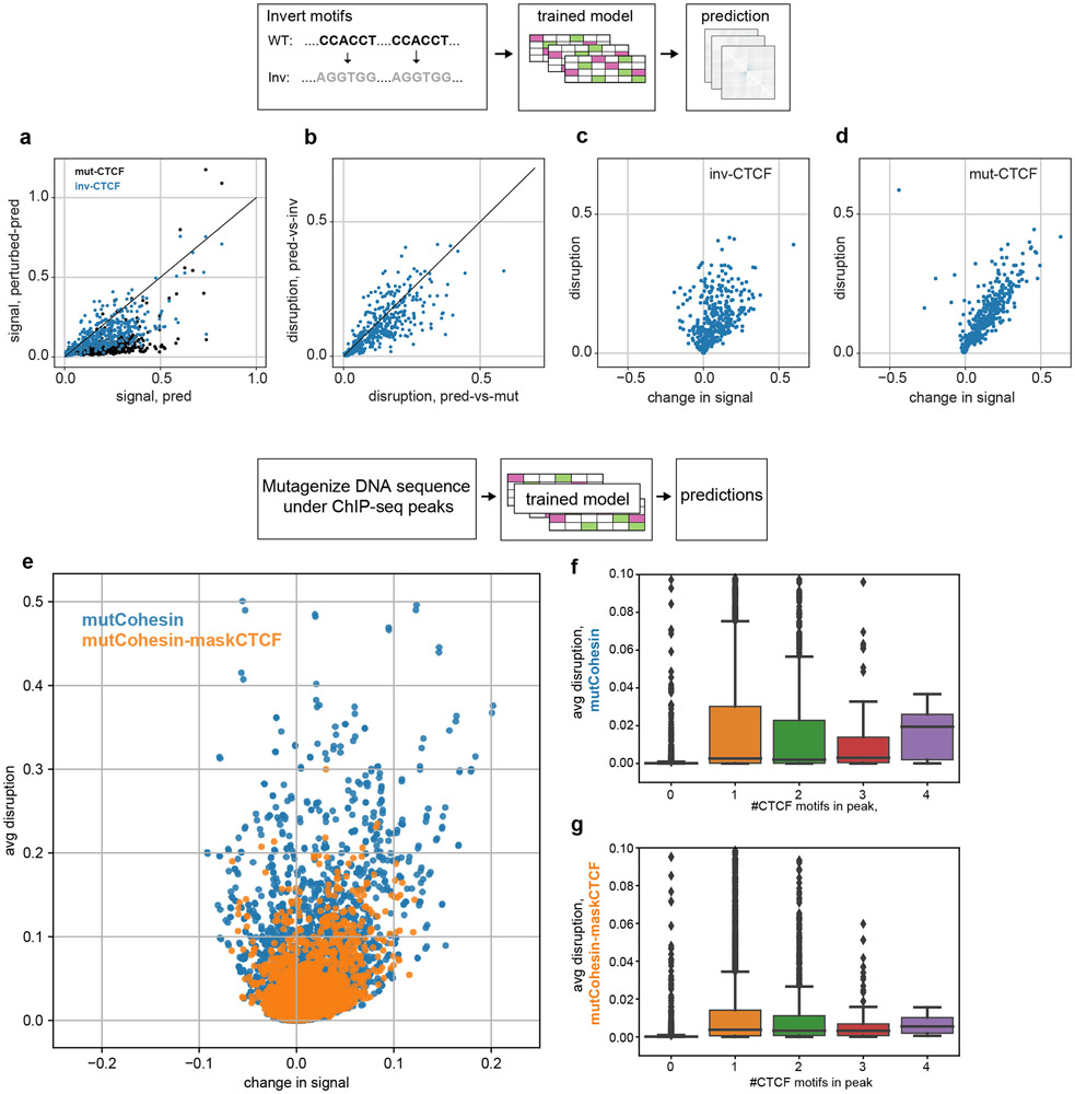
Akita predicted more prominent patterns in regions with greater CTCF binding and DNAse hypersensitivity (Extended Data Fig. 3a-c). Salient predicted patterns often also aligned with CTCF ChIP-seq peaks (Fig. 2a,b). However, CTCF motifs are too prevalent to connect DNA sequence to genome folding at the bin level (Extended Data Fig. 5d). Fortunately, Akita enabled us to directly quantify nucleotide influences via in silico mutagenesis; while training Akita was computationally intensive, effects of sequence changes could be predicted in seconds. Akita predicted greatly diminished locus-specific patterns after mutating all CTCF motifs (Fig. 2e). In this extreme scenario, Akita predicted some patterns would persist, and these often aligned with DNase hypersensitive sites that lacked evidence of strong CTCF binding. Inverting all CTCF motifs produced very different predictions, redistributing rather than abrogating contact patterns (Fig. 2d, Extended Data Fig. 6a-d). This indicated that Akita learned an orientation-specific grammar of the CTCF sites most crucial for genome folding.
Figure 2: Akita predictions relate to CTCF binding and genome accessibility.
a. Log(observed/expected) target HFF maps for three different genomic regions in the test set, binned to 2048bp.
b. Binned profiles at 2048bp for CTCF ChIP-seq fold-change over control and DNAse density, downloaded from the ENCODE data portal37.
c. Predictions for the same three regions.
d. Predictions for inverting all CTCF motifs in each region. Note that patterns are perturbed relative to (c), and have greater saliency as compared with (e).
e. Predictions for random mutagenesis of all CTCF motifs within each region, averaged over ten instances. Grey shading shows regions with CTCF binding (from b) that are disrupted in these maps, and yellow shading shows regions with high DNAse but low levels of CTCF binding that are boundaries of residual structures after CTCF motif mutagenesis.
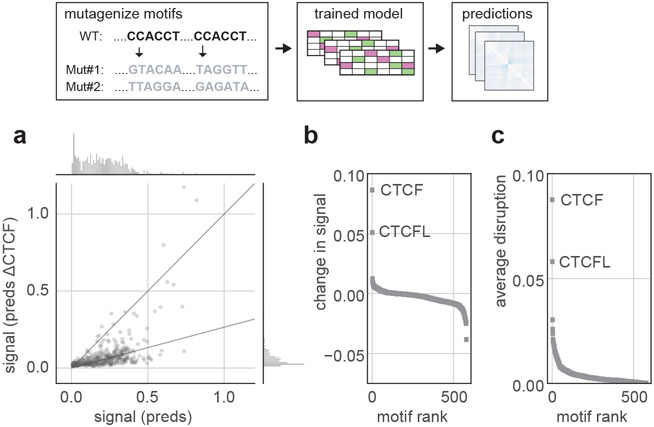
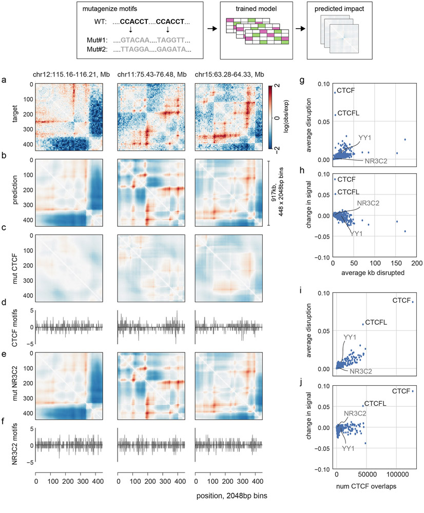
To explore the role of CTCF for Akita’s predictions genome-wide, we mutagenized the CTCF motifs in each region of the test set. The majority of mutagenized regions showed weaker locus-specific patterns (Fig. 3a), reminiscent of changes seen experimentally following acute CTCF degradation22,23. Performing a similar mutagenesis for each motif in the JASPAR transcription factor database24 revealed that CTCF had the strongest impact (Fig. 3b,c). The second largest effect was for CTCFL, which binds a very similar motif to CTCF but is typically inactive in somatic cells. For the remaining motifs, mutagenesis either imperceptibly disrupted genome folding or the predicted impact directly tracked the number of overlaps with CTCF motif positions (Extended Data Fig. 5g-j). Going beyond motifs, we also explored the effect of mutating sequences underlying cohesin ChIP-seq peaks. This analysis indicated that DNA sequences other than the core CTCF motif can also impact genome folding (Extended Data Fig. 6e-g).These results argue that no other transcription factor with a known motif plays as large of a role as CTCF for 3D genome folding, and that CTCF-independent aspects of genome folding emerge from a combinatorial interplay between different DNA-binding factors.
Figure 3: Akita reveals large impacts of CTCF motif disruptions on genome folding.
a. Predicted map signal strength before versus after mutagenizing all CTCF motifs, for each region in the test set for the HFF model output. Map signal strength is measured as mean((pred)2). Motifs are mutagenized by replacing the DNA sequence at each position in each motif with randomly generated nucleotides. Akita predicts that mutagenizing CTCF motifs leads to more uniform maps, shown by the lower dynamic range after mutagenesis, mean((predΔCTCF)2), confirming the visual trend seen in Fig. 2e across the test set.
b. Change in map signal strength, measured by the difference of the mean squared values before versus after mutagenizing each motif in JASPAR24, mean((pred)2) - mean((predΔmotif)2). Positive values indicate lower signal after mutagenesis, as for CTCF.
c. Average disruption, measured by the mean-squared differences between predictions before versus after mutagenizing each motif in JASPAR, mean((pred- predΔmotif)2). By this metric, CTCF mutagenesis is more than three times as impactful as mutagenesis of any other motif besides CTCFL. Note high scores for other motifs are likely driven at least in part by frequent overlaps with CTCF motifs (Extended Data Fig. 5).
Akita learns predictive nucleotide-level features of genome folding
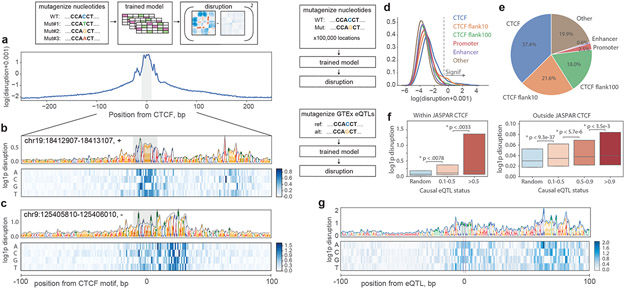
Given the substantial predicted impact of mutagenizing whole CTCF motifs on genome folding, we sought to quantify the predicted contact map disruptions for mutations to individual nucleotides. First, we performed in silico saturation mutagenesis of 500-bp regions centered at strong CTCF motifs (JASPAR p-value < 1e-6). Predicted disruptions were largest for nucleotides around the motif, but remained high relative to background in the flanking regions, slowly decaying with increasing distance (Fig. 4a-c). The magnitude of predicted disruption correlated with evolutionary conservation (phyloP25, Extended Data Fig. 7a-c) and predicted change in motif strength from FIMO26 (Extended Data Fig. 7d). We next generated 100,000 random single nucleotide mutations uniformly spaced across the 241Mb test set to quantify the influence of nucleotides within and near CTCF motifs relative to other genomic features. Mutations that altered CTCF motifs and their flanking regions displayed many of the highest predicted disruption scores (Fig. 4d,e, Extended Data Fig. 7e-f), which likely reflect influences on CTCF binding or function, either directly or via cofactors27,28. Nucleotides in promoters and enhancers also displayed elevated effects relative to genomic background. Still, a substantial fraction (19.9%) of high-impact mutations fell outside of annotation categories typically considered in connection with 3D genome folding. These analyses indicate that Akita extracts meaningful information at the base pair level, and that important DNA sequences for genome folding remain uncharacterized.
Figure 4: Akita extracts informative nucleotide-level features of genome folding.
a-c. Saturation mutagenesis around CTCF motifs. a. Mean disruption scores calculated from saturation nucleotide-level mutagenesis of 500bp regions around 500 randomly selected high-quality CTCF motifs (JASPAR p-value < 1e-6) in the test set sequences. Before averaging across the 500 sequences, we constructed a single score for each position by taking the maximum across alternative alleles, added a 0.001 pseudocount to stabilize values for visualization, and computed the logarithm. The motif position is indicated in grey.
b,c. Example sites with high disruption scores in flanking regions. Visualizations include a 1 pseudocount preceding the logarithm (log1p) to make all scores positive. Heatmaps show scores for each possible nucleotide substitution. Nucleotide letter heights are drawn proportional to the max across three possible substitutions per position.
d,e. Unbiased genome-wide mutagenesis. d. Distributions of disruption scores for 100,000 unbiased mutations across the test set, split by annotation category. Pseudocount and log scale as in (a). Vertical dashed line indicates threshold for mutations considered in (e).
e. High disruption mutations (top 356 from (d)) split by annotation category, excluding previous categories in the hierarchy. Categories are considered hierarchically counter clockwise, starting from those that influence CTCF motifs (CTCF, Flank10, Flank100, Promoter, Enhancer, Other). Flank10 and Flank100 represent nucleotides falling within 10 or 100bp of a CTCF motif (see Extended Data Fig. 7 for additional detail). This conservative categorization provides strong evidence for the contribution of nucleotides beyond canonical CTCF motifs for genome folding.
f,g. GTEx eQTL mutagenesis.
f. Distribution of disruption scores for GTEx eQTL variants falling inside (left) and outside (right) JASPAR CTCF motifs, stratified by casual posterior probability. Boxes represent interquartile ranges, with median marked. Random indicates the distribution for a set of control SNPs with significant genome-wide marginal association with gene expression. Within CTCF, the bar plots represent 57 SNPs with causal posterior probability (PP) >0.5, 138 SNPs with PP from 0.1 to 0.5, and 58 random SNPs with significant genome-wide marginal association with gene expression. Outside CTCF bar plots represent 1,873 SNPs with PP>0.9, 1,820 SNPs with PP from 0.5 to 0.9, 15,926 SNPs with PP from 0.1 to 0.5, and 8,885 random genome-wide significant SNPs. We compared SNP scores with one-sided Mann-Whitney U tests to produce the p-values displayed.
g. Saturation mutagenesis around a high-scoring non-CTCF variant: chr7_5898574_G_T_b38, which acts as an eQTL of CCZ1 with high probability. The SNP affects an AGCCCTCTCCTGTA motif that is unrecognizable by the TomTom motif search tool38, but lies 70 bp away from a CTCF motif, and may serve to influence its boundary capabilities. Heatmap and letter heights as in (b).
To consider how genome folding influences gene expression, we studied a set of fine-mapped likely causal expression quantitative trait loci (eQTLs) from GTEx whole blood samples (Fig. 4f). Using Akita, we calculated the predicted disruption to local 3D folding (averaged across the five model outputs) for single nucleotide polymorphisms (SNPs) at varying causal posterior probability (PP) thresholds (1,906 PP>0.9, 29,112 total). We observed significantly larger predicted disruptions for SNPs with greater causal PP, both overlapping and outside of CTCF motifs (Fig. 4f). To characterize the sequence context around these high-scoring non-CTCF variants, we performed in silico saturation mutagenesis of the surrounding 200 bp. One intriguing example altered an uncharacterized motif 70 bp from a CTCF motif, which may serve to enhance its boundary strength (Fig. 4g). These results show how Akita can be used to interpret human genetic variation.
Akita predicts consequences of a genetically engineered deletion
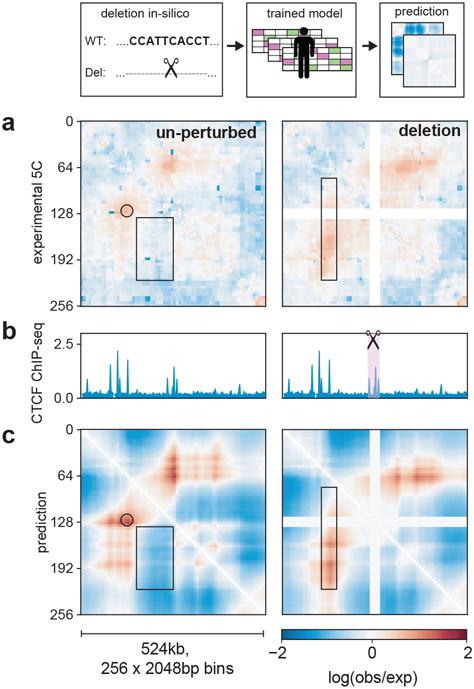
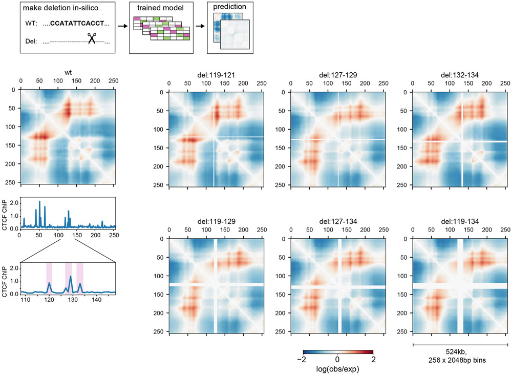
We investigated Akita’s ability to predict how genetically engineered mutations alter genome folding. As Akita makes predictions for 1Mb sequences and is not influenced by information beyond this window, we sought an example where a <100kb variant had a dramatic effect on genome folding. At the Lmo2 locus in HEK293T cells29, two domains are separated by a boundary positioned at a cluster of three CTCF-bound sites (Fig. 5). In cells with a ~25kb deletion encompassing this boundary, the two domains merge. Making the same deletion in silico recapitulated this effect in the predicted Hi-C map. Leveraging Akita’s ability to rapidly assay sequence perturbations, we examined a combinatorial set of in silico deletions in the Lmo2 locus (Extended Data Fig. 8). Deleting any individual CTCF site minimally altered predictions. Our model thus predicts this boundary is formed by redundant CTCF sites, a phenomenon observed experimentally in other genomic locations4,5.
Figure 5: Predicting a genetically engineered deletion with Akita.
a. Experimental29 log(observed/expected) 5C data in HEK293T cells for WT (left) and a CRISPR/Cas9-mediated deletion of a ~25kb boundary region (right) at the Lmo2 locus for a 219 bp region centered at the deleted boundary (chr11:33752474-34276762). In wild-type cells (left), this region displays a peak at the boundary (circle) between two ~130kb domains that are relatively insulated from each other (rectangle), separated by a boundary that overlaps a cluster of three CTCF-bound sites. In cells where this boundary has been deleted (right), the two domains merge and display a flare of enriched contact frequency (thin rectangle).
b. CTCF profiles for HEK293T29.
c. Computational predictions for WT (left) and deletion (right) of the boundary, using the HFF output from our human-trained model, showing similar changes. Views centered at the middle of the full predicted window to highlight the region with changes.
Akita enables cross-species analyses of genome folding
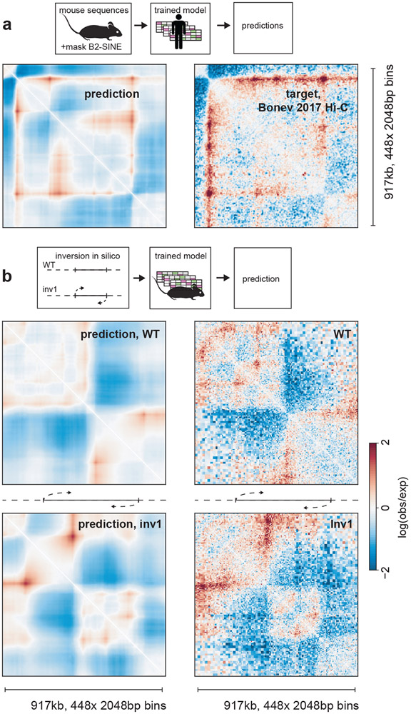
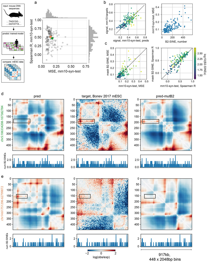
Given similar overall human and mouse genome folding30, we reasoned the mouse genome could provide evolutionarily perturbed sequences to further test Akita (Fig. 6a). Using mouse DNA sequences as input, we compared predictions from our human-trained model (hESC output) with mESC Hi-C data31. These cross-species predictions generally recapitulated mouse genome folding (Extended Data Fig. 9, median Spearman R: 0.50). Intriguingly, poorer predictions had more B2 SINE elements, which dramatically expanded in murid lineages and carry CTCF sites32. Mutagenizing B2 SINE elements to ablate their CTCF sites improved our predictions for mouse genome folding (median Spearman R 0.55 vs 0.50). This suggests that the mouse genome specifically mitigates the influence of these elements, and Akita did not learn their true influence due to the lack of B2 SINEs in the human genome training data.
Figure 6: Akita learns species-specific relationships between DNA sequence and genome folding.
a. Predicting mouse genome folding with a human-trained model. Left: computational prediction for mouse genome folding, using the hESC output from our human-trained model after mutagenizing B2 SINE elements. Right: experimental mESC Hi-C data31 for the same region.See Extended Data Fig. 9 for quantification across the mouse genome.
b. Predicting a genetically engineered inversion with a mouse-trained model.
Left: Akita predictions from WT DNA sequence (top) and DNA sequence with the inversion (bottom) at the Eph4A locus. Right: Experimental capture-C data for WT (top) and a ~622kb inversion (bottom, Inv1) at the Eph4A locus34. Predictions were generated using a mouse-trained model and the mESC output, and show similar changes to those observed experimentally. See Extended Data Fig. 10 for comparison between mouse-trained and human-trained models.
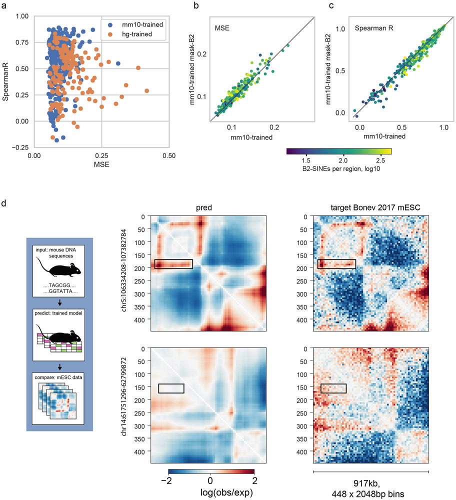
To test whether the influence of B2 SINEs on mouse genome folding could be learned de novo via our approach, we trained a new model on available mouse Hi-C data (Extended Data Fig. 10). This model was both more predictive on held-out test regions of the mouse genome for the same mESC Hi-C data (median Spearman R 0.63 vs. 0.50 for the human-trained model), and was not improved by mutating B2 SINE elements (median Spearman R 0.62 masked vs 0.63 unmasked), indicating that it correctly learned to mitigate the impact of CTCF sites inside of these elements. Our results are consistent with recent observations that the ChAHP complex hinders CTCF binding within murine B2 SINE elements33, and highlight opportunities for sequence-based modeling to uncover species-specific regulatory strategies.
To further test the generality of our approach, we considered the ability of our mouse-trained model to predict a genetically engineered inversion. At the Eph4A locus in limb buds, two domains are separated by a boundary with a prominent downstream flare34. Upon inversion of ~622kb encompassing this boundary and a downstream enhancer, the orientation of the flare flips, as ascertained by Capture-C at this locus34. Making the same inversion in silico, we found a similar change in the predicted contact maps (Fig. 6b). Note that as high-resolution limb bud data was unavailable for model training, we used the mESC output from our model. This result illustrates the generality of our approach, for both a new organismal context (mouse instead of human) and class of structural variant (inversion instead of deletion).
Discussion
In summary, we present Akita, a convolutional neural network model that predicts 3D genome folding using only DNA sequence as an input. We demonstrated how Akita enables rapid in silico mutagenesis at the motif and single nucleotide level, and how this allows for interpreting the features used in its predictions. We further show how Akita can be used to interpret eQTLs from GTEx and make predictions for multi-kilobase structural variants. Finally, we highlighted how our approach can uncover species-specific influences of sequence on genome folding.
While Akita advances predictive modelling of genome folding, our current implementation makes predictions for ~1Mb windows of the genome and, crucially, is not influenced by information beyond this window. Future work will be needed to extend predictions to more distal pairs of genomic loci and model features of genome folding visible between chromosomes, like A/B compartmentalization1. As Akita takes a data-driven approach, it must be trained using Hi-C or Micro-C data for any cell types where sequence perturbation predictions are desired. Future work, which can include new training strategies, network architecture modifications, and leveraging additional datasets, will also be necessary to sharpen cell-type specificity of predictions. The increasing availability of high-resolution Hi-C and micro-C data promises an exciting path forward.
An appealing hypothesis for future work is that neural networks with layers that better reflect the molecular and physical mechanisms organizing genomes will make more accurate and generalizable predictions. For the initial layers, convolutions naturally extend13-15 position weight matrix approaches for capturing the biophysics of protein-DNA interactions. The architectures and layers that might best reflect the process of loop extrusion, believed to organize mammalian interphase chromosomes3, or other mechanisms of genome organization remain open questions. The near future promises exciting progress: recently, a similar CNN model, deepC, was posted to bioRxiv35. While deepC has a similar ‘trunk’ to Akita, it differs greatly in the architecture of the ‘head’, data pre-processing, and training schemes (Supplemental Note 3). Future work will benefit from comparing these approaches, continuing to explore the space of alternatives, and incorporating high quality data as it becomes available.
In the future, we envision that end-to-end sequence-to-genome-folding approaches will advance our ability to design functional screens, model enhancer-promoter interactions, prioritize causal variants in association studies, and predict the impacts of rare and de novo variants.
Online Methods
Training Data
To obtain Hi-C data conducive for convolutional neural network learning, we reprocessed five of the highest-quality publicly available human Hi-C and Micro-C datasets to 2048bp (211 bp) bins using distiller (https://github.com/mirnylab/distiller-nf)44 to map to hg38 and cooler (https://github.com/mirnylab/cooler)45 to perform genome-wide iterative correction (ICE) 20.
To focus on locus-specific patterns and mitigate the impact of sparse sampling present in even the currently highest-resolution Hi-C maps, we adaptively coarse-grain, normalize for the distance-dependent decrease in contact frequency, take a natural log, clip to (−2,2), linearly interpolate missing bins, and convolve with a small 2D gaussian filter (sigma=1, width=5). The first through third steps use cooltools functions (https://github.com/mirnylab/cooltools). Interpolation of low-coverage bins filtered out in typical Hi-C pipelines was crucial for learning with log(observed/expected) Hi-C targets, greatly outperforming replacing these bins with zeros.
To prepare input DNA sequences with paired Hi-C data for training, we divided the human genome into non-overlapping virtual contigs and assigned them randomly to training, validation, and test sets with an 80/10/10 split. To generate the set of virtual contigs, we split chromosomes at assembly gaps, large unmappable regions, and consecutive stretches of ≥10 filtered-out Hi-C bins (in any target dataset). The resulting segments were split into 10 Mb virtual contigs. From the contigs we extracted 220 bp (~1Mb) sequences, striding by 218 bp (~262kb) for the training set and 219 bp (~524kb) for the validation and test sets. This procedure resulted in 7,008 training, 419 validation, and 413 test sequences.
Model architecture
We created a neural network architecture to predict 2D Hi-C maps from 1D DNA sequences that consists of two major components. First, we process the 1D DNA sequence using a ‘trunk’ that applies a series of convolutions, following previous work on convolutional neural networks for DNA sequence analysis. Second, we applied a ‘head’ that transforms the 1D representations to 2D for Hi-C prediction. Importantly, we make a prediction for each dataset the model is trained on for a given input DNA sequence. Intriguingly, similar sequence-to-map architectures have recently been successful for protein contact map prediction48. We implemented the model using the Basenji software18,19, which is written in Tensorflow49 and Keras50.
More specifically, the ‘trunk’ includes:
Convolution with 96 filters of size 11-by-4 to transform the 1-hot encoded DNA sequence followed by batch normalization, ReLU, and width 2 max pooling.
Convolution tower that iteratively performs convolution with 96 filters of width 5, batch normalization, ReLU, and width 2 max pooling to arrive at 512 vector representations of the sequence in 2048bp windows.
Dilated residual convolution tower that iteratively performs dilated convolution with geometrically increasing dilation rate, adding the new representation back into the old. This block spreads information about relevant sequence elements and global context across the sequence18. As previously18, dilated convolutions use zero padding. Dropout is applied before adding the new representation back to the old at each iteration.
Bottleneck width 1 convolution with 64 filters.
The ‘head’ includes:
Conversion of 1D profiles to 2D maps. We averaged the representations for every pair of genomic bins i and j. This operation transforms a tensor with dimensions [512 length, 64 filters] to a tensor with dimensions [512 length, 512 length, 64 filters]. We also concatenated a positional encoding of the distance between bins, abs∣i-j∣, as an additional filter, producing a [512 length, 512 length, 65 filters] tensor. We then applied a (1,1) convolution block to finalize the transition to 2D.
2D dilated residual convolution tower that iteratively performs dilated convolution, treating this map as a 2D image as adding the new representation back to the old at each iteration. As above, we use geometrically increasing dilation rate, and dropout. We additionally re-symmetrize at each iteration with the custom Keras layer Symmetrize2D, which sums the output of a layer with its transpose and divides by two.
Linear transformation, without any activation, to make simultaneous predictions for the 5 datasets.
Collectively the model has 746,149 trainable parameters. For the full Keras print of the model architecture see: [https://github.com/calico/basenji/blob/master/manuscripts/akita/keras_print.txt].
Training Approach
We computed a mean squared error loss from the targets and predictions, considering only the upper triangular portion of the matrixes. We fit the model parameters using stochastic gradient descent with momentum for ~60 epochs, taking steps in batches of 2 sequences.
Data augmentation was critical to avoid overfitting and maximize generalization accuracy to unseen sequences. Each time that we processed a sequence, we stochastically shifted input sequences by up to +/− 11 bp and reverse complemented the DNA and flipped the Hi-C map.
We stopped training when validation loss had not improved for 12 epochs, and we took the model parameters that had achieved that minimum validation loss forward as the final model. We performed a search over learning rate, momentum, gradient norm clipping, dropout probability, and convolution filters using the Dragonfly Bayesian optimization toolkit [https://github.com/dragonfly/dragonfly]51. Best performance was achieved with learning rate: 0.0065, momentum: 0.99575, gradient clipping: 10.7. Full specification of model parameters can be found at: [https://github.com/calico/basenji/blob/master/manuscripts/akita/params.json].
Comparison with 1D features
For comparison to 1D features of the epigenome, we downloaded processed bigWigs for the relevant cell types from the ENCODE data portal 37 and binned them into 2048bp profiles.
In silico motif mutagenesis
To perform in silico motif mutagenesis, we intersected our test set regions with motif positions using bedtools 52. We then generated multiple randomized sequences, where we replaced the DNA sequence at the motif positions with randomly generated nucleotides of the same length. We then calculated the average disruption as mean( (pred - predΔmotif)2 ), and the change in signal as mean(pred2 ) - mean(pred2Δmotif). Motif names were plotted with adjustText [https://github.com/Phlya/adjustText]53. The maps in Fig. 2 represent averages over 10 randomized sequences, while the JASPAR-wide analyses in Fig. 3 averaged over 3 randomized sequences.
In silico CTCF motif inversions
We performed in silico motif inversions similarly to motif mutagenesis for determining intersections. We then merged overlapping motifs and replaced sequences in these intervals with their reverse complements.
In silico nucleotide-level mutagenesis.
We studied the impact of CTCF with two nucleotide-level mutagenesis strategies. First, we performed saturation mutagenesis of 500 bp regions around 500 randomly selected strong CTCF motifs, annotated by JASPAR with p-value < 1e-6. Second, to quantify the impact of nucleotides within and near CTCF motifs relative to other genomic features, we formed a set of unbiased mutations across the genome. We selected 100,000 uniformly spaced positions (each 256 bp apart) within the test set genomic regions and then selected a random alternative nucleotide for each one. For each of these mutagenesis strategies, we computed the disruption score as the L2 norm of the predicted difference between contact maps for the reference and alternative allele, averaging across outputs.
In silico GTEx mutagenesis.
We studied fine mapped GTEx v8 eQTLs54 from whole blood using SuSiE55, including 1,906 SNPs with causal posterior probability (PP) >0.9, 1,844 SNPs with PP from 0.5 to 0.9, and 16,064 SNPs with PP from 0.1 to 0.5. We further selected 9,298 random SNPs with significant genome-wide marginal association with gene expression. We computed disruption scores with Akita by predicting contact maps for the reference and alternate alleles, subtracted the maps and computing the L2 norm as for in silico nucleotide-level mutagenesis
Human-trained predictions for mouse DNA sequences
To test the accuracy of Akita’s predictions for mouse DNA sequences, we obtained mESC Hi-C data from Bonev et al., 2017 31, mapped reads to mm10, and otherwise processed the data as for human datasets. Positions of B2 SINE elements were downloaded from UCSC (from RepeatMasker42). B2 SINE mutagenesis was performed as described for motifs.
Mouse model training
We trained a mouse (mm10) model using Hi-C data from Bonev et al.31 (mESC, CN, ncx_CN, NPC, ncx_NPC) and Micro-C from Hsieh et al.43 (mESC) with the same multi-task framework used to train our hg38 model.
5C and Capture-C data processing
To test Akita’s ability to predict an experimentally induced deletion, we obtained processed 5C data for the Lmo2 locus from Hnisz et al., 201629, re-binned fragments to 2048bp bins, and otherwise performed the same processing into log(observed/expected) maps as for Hi-C target data above.
To test the ability of our mouse-trained model to predict an experimentally induced inversion, we obtained processed Capture-C data for the Eph4A locus from Kraft et al., 201934. Mapped experimental data was re-binned to 2048bp with cooler45, iteratively corrected in cis with a minimum of 100 reads, and then processed into log(observed/expected) maps as described for Hi-C target data above.
In silico deletions and inversions
As Akita makes predictions for fixed input size, to make a deletion in silico we must both remove the DNA sequence we hope to delete and supply the model with an equal amount of additional DNA sequence. Here we centered on the position of the deletion and symmetrically extended the start and end to maintain the size of the input. For inversions in the window, as considered here, we simply replaced sequence in this region with its reverse complement.
Statistics and software
The statistical tests in comparisons are indicated in the main text and figure legends. Pearson R, Spearman R, one-sided Mann-Whitney U tests calculated using scipy56 v1.4.1. Analyses also used numpy57, pandas58, ipython59, matplotlib60 and seaborn61. Additional information available in the Life Sciences Reporting Summary.
Data availability
Datasets analysed in this study are publicly-available from: GEO (www.ncbi.nlm.nih.gov/geo/, Hi-C: GSE63525, GSE104334, GSE96107, 5C: GSE77142, Capture-C: GSE116794), 4D Nucleome Data Portal (https://data.4dnucleome.org/, Micro-C: 4DNESWST3UBH, 4DNES14CNC1I), UCSC (http://hgdownload.cse.ucsc.edu/goldenpath/hg38/database/), ENCODE data portal (www.encodeproject.org/), JASPAR (http://expdata.cmmt.ubc.ca/JASPAR/downloads/UCSC_tracks/2018/hg38/tsv/), GENCODE (https://www.gencodegenes.org/human/), FANTOM5 (https://fantom.gsc.riken.jp/data/).
Code availability
Trained model, additional documentation, and code for training and predicting with Akita available at: https://github.com/calico/basenji/tree/master/manuscripts/akita.
Extended Data
Extended Data Fig. 1. Akita transforms from 1D to 2D representations and benefits from multi-task training.
a. Illustration of transformation from 1D profiles to 2D maps. To convert 1D profiles to 2D maps, we averaged the values at pairs of genomic bins i and j for each filter. This operation transforms a tensor with dimensions [512 length, 64 filters] to a tensor with dimensions [512 length, 512 length, 64 filters]. We also concatenated a positional encoding of the distance between bins, abs∣i-j∣, as an additional filter, producing a [512 length, 512 length, 65 filters] tensor.
- “dot”: Element-wise multiplication between each vector position, t(i,j,k) = oi(k)oj(k).
- “geo”: Addition of one to all vector values, element-wise multiplication between each position, square root of each position, subtraction of one from all vector values,
- “max”: Element-wise max between each vector position, t(i,j,k) = max(oi(k),oj(k)).
- “concat”: Concatenate the two vectors, t(i,j) = [oi,oj].
- “avg”: Element-wise mean between each vector position, t(i,j,k) = (oi(k)+oj(k))/2
c. Multi-task training improves accuracy relative to single dataset training.
We trained Akita models for each of the five datasets alone and compared overall Pearson’s R on the test set to the jointly trained multi-task model. Multi-task training benefitted all datasets except for the highest-performing H1hESC dataset. We note that our multi-task framework thus offers a powerful approach to train on many datasets simultaneously and efficiently.
Extended Data Fig. 2. Correlation of Akita’s predictions with experimental data reach those between replicates.
a. MSE vs. Spearman R for each target, where each dot shows values for these metrics for an individual region of the test set. Light grey shows values for predictions versus the full experimental dataset, as in Fig. 1C. Purple shows these quantities if reads for each full dataset are randomly split into two datasets. The same normalization and smoothing steps used to generate training data from the full dataset were used to transform each map prior to calculating MSE or Spearman R. Predictions generally show lower MSE and higher correlations than split datasets. This indicates that our model has extracted the majority of the signal in these data, and that current performance is limited at least in part by sequencing depth of even the currently best available datasets.
b. MSE vs. Spearman R for the HFF dataset. Light grey and purple as in (a). To obtain contact maps for biological replicates, as defined in Krietenstein et al., 2020, reads were re-processed and aggregated across technical replicates for the same biological replicate (bioRep). Biological replicates represent independently cultured and processed cells, whereas technical replicates represent independent sample preparations from the same cell culture. Green shows results for two biological replicates, and dark grey shows results for predictions versus the first biological replicate. Normalization and smoothing applied as in (a). Since splitting leads to slightly lower MSEs and higher correlations than those between biological replicates, this indicates that splitting reads in half computationally leads to a similar, albeit more stringent, barometer of model performance than the comparison between biological replicates.
c. Maps for predictions (top row), bioRep1 (middle) and bioRep2 (bottom) for the same three regions displayed in Fig. 2.
Extended Data Fig. 3. Akita predictions relate to the aggregate CTCF and accessibility signals as well as binarized features of experimental maps.
a-c. Correlations between the strength of Akita’s predictions, strength of experimental patterns, CTCF, and DNAse.
a. Map signal strength, measured by mean of squared map values, for predictions versus targets. In regions with more complex features, Akita tends to make more complex predictions. Correlation printed above each plot indicates Spearman’s R across all regions of the test set (n=413, p<1e-6 in all cases).
b. Signal strength for predictions versus signal strength for CTCF ChIP-seq, measured by mean squared profile values. Akita predicts more prominent locus-specific patterns in regions with greater CTCF binding.
c. Signal strength for predictions versus DNAse-seq.
d-f. Akita predictions recapitulate positions of boundaries and dots called from experimental data.
d. Experimental HFF Micro-C data for the same regions in Fig. 2. TAD boundaries are overlaid as green lines, for boundary strength >1 and insulation score < −0.5 (15,273 genome-wide). Dots (also termed ‘loops’ or ‘peaks’) are overlaid as purple circles, for strength >2 (36,671 dots genome-wide). Both calculated as in Krietenstein et al., 202036.
e. Predictions overlaid with the same features.
f. A/B compartment profiles for the indicated regions calculated at 32,768bp (215) resolution, calculated using cooltools (https://github.com/mirnylab/cooltools) from chromosome-wide experimental maps. Note that these 1 Mb regions all largely fall in the A-compartment (values >0), and that B-compartment regions often display the more uniform maps seen in Fig. 1b. Also note that called TAD boundaries and peaks likely have both false positives and false negatives, as derived features extracted by related algorithms from the same Hi-C data can show surprisingly low overlap12, and are dependent on the exact thresholds used. Indeed, binarized features alone appear to have minimal predictive value for functional enhancer interactions in CRISPRi tiling screens39. The limitations of binarized features underscores a key goal for Akita, which is to enable post-TAD analyses of genome folding data.
Extended Data Fig. 4. Akita displays limited cell-type specificity in predictions.
a. Predicted versus experimental log(observed/expected) values for each bin pair in every region of the test set, separately for each target. This shows predictions are correlated with experimental data across cell types. Color shows log10 number of bin pairs for each set of predicted versus experimental values. Corr shows Spearman R.
b. Considering every region in the test set across cell types, we find: Left: models make highly correlated predictions for different cell types (Spearman R(pred(i,j,k1),pred(i,j,k2)), where k1 and k2 index cell types and the correlation is taken across all genomic regions i, and pixels j). Middle: genome folding assayed experimentally is correlated, but less so (Spearman R(data(i,j,k1),data(i,j,k2)). Right: predicted differences across cell types from our models correlate, albeit weakly, with observed differences (Spearman R((pred(i,j,k1) - pred(i,j,k2), data(i,j,k1) - data(i,j,k2)). Note different scales for Spearman R.
c. Example of a region showing largely consistent folding across cell types (chr20:50759680-51808256) for targets and predictions. Tracks show binned CTCF ChIP-seq fold-change over control and DNAse-seq density.
d. Example of a region showing gains and losses of specific features across cell types (chr5:5179392-6227968) at bin ~300.
While the predicted differences across cell types from models correlates with observed differences (b, right), our predictions are not particularly visually distinct for different cell types (c,d). At present, our models appear to primarily tune the dynamic range for the entire prediction, rather than predicting gains and losses of a subset of features (d). Also note in (d) that CTCF is still bound in HCT116 in this region as determined by ChIP-seq, despite the loss of a strong boundary around bin 300. In the future, we hypothesize that pairing improved model architectures and training procedures with a greater number of high-resolution genome folding datasets will enable our models to learn more cell type-specific representations of genome folding, as is currently possible for TF binding, chromatin state, and gene expression18.
Extended Data Fig. 5. In silico mutagenesis enables rapid screening of transcription factor influence on genome folding.
a. Experimental HFF Micro-C target data for three regions in our held-out test dataset.
b. Predictions for these regions.
c. Predictions for these regions after randomly mutagenizing all CTCF motifs in these regions, averaged over 10 random samples.
d. Number of CTCF motifs per 2048bp bin. CTCF motif matches obtained from JASPAR24, and profiles computed separately for the number of motifs on the positive strand (>0) and negative strand (<0).
e. Predictions for these regions after mutagenizing all NR3C2 motifs in these regions, averaged over 10 random samples. NR3C2 motifs cover a similar number of base pairs per region as CTCF, but their perturbation has little impact on Akita’s predictions.
f. Positions of positively oriented (>0) and negatively (<0) oriented NR3C2 motifs per bin.
g. Average disruption, mean( (pred-predmut)2), versus the average number of kb perturbed per region. Note that YY1, suggested to be involved in genome folding40,41, is predicted to have little aggregate genome-wide impact following motif mutagenesis. This suggests YY1 may operate at a subset of loci in certain developmental contexts40 or its influence depends on the presence of nearby CTCF motifs or other complex factors and evaded our model.
h. Change in signal, mean((pred)2) - mean((predmut)2), versus the average number of kb perturbed per region. This reveals a trend toward negative scores for motifs with many occurrences.
i. Average disruption versus the total number of overlaps with CTCF motifs. The strong trend argues that many high scoring motifs likely have large predicted impacts due to frequent overlaps with CTCF motifs, rather than independent effects.
j. Change in signal versus the total number of overlaps with CTCF motifs.
Extended Data Fig. 6. Akita learns an orientation-specific role for CTCF and enables mutagenesis of regions defined by ChIP-seq.
a-d. Akita learns an orientation-specific role for CTCF
a. Predicted map signal strength before versus after in silico perturbations, either for mutagenizing all CTCF motifs (black) or inverting all CTCF motifs (blue). Points show each region in the test set (n=413). Signal strength quantified by mean squared map values. Inversions tend to show smaller perturbations to overall signal strength (blue points deviate less from the x=y line than black points).
b. Average disruption for mutagenizing all CTCF motifs or inverting all CTCF motifs. Inversion disrupts maps to a similar extent as mutagenesis (points fall both above and below the x=y line to a similar extent). Jointly with (a), Akita thus predicts changing motif orientation largely alters the positioning of contact patterns, rather than their overall salience across the genome.
c. Change in signal strength versus disruption for inverting all CTCF motifs, mean((pred)2) - mean((predinv-CTCF)2). Points show each region of the test set. This indicates that while motif inversions greatly change predicted contact patterns, they can both increase (-) and decrease (+) the signal strength, or salience, of contact patterns.
d. Change in signal strength versus disruption for mutagenizing all CTCF motifs in each region of the test set, mean((pred)2) - mean((predmut-CTCF)2). The positive change in signal strength upon mutagenesis shows these perturbations largely decrease features strength in predicted maps.
e-g. Akita enables studying the impact of sequences underlying ChIP-seq regions without defined motifs.
e. Predicted change in signal versus average disruption for in silico mutagenesis of DNA sequences underlying cohesin peaks. Each point represents one of the 10,268 H1hESC Rad21 cohesin peaks overlapping regions in our test set. Mutagenesis is performed either randomly for all nucleotides under the peak (blue) or only for nucleotides that do not overlap a Jaspar CTCF motif (orange).
f. Boxplots for predicted average disruption, stratified by the number of CTCF motifs overlapping the cohesin ChIP peak. Boxplots generated with seaborn defaults for the same n=10,268 peaks (boxes show quartiles, whiskers extend 1.5 times IQR beyond low and high quartiles, points outside this range shown individually). We found that mutagenesis of Rad21 ChIP-seq peaks without CTCF motifs was less disruptive than mutagenesis of peaks with CTCF motifs. Interestingly, we observed no clear trend of increased average disruption for increased numbers of CTCF motifs beyond the first.
g. Boxplots as for (f) but with masking the positions of CTCF motifs in these peaks and repeated mutagenesis. On average this led to weaker disruptions of predicted maps (also see the spread of orange versus blue in (e)). However, the trend where mutagenesis of Rad21 ChIP-seq peaks without CTCF motifs was less disruptive than mutagenesis of peaks with CTCF motifs still held. This argues that Akita relies on additional sequence context beyond the immediate 19bp motif in JASPAR to correctly predict its impact on Hi-C maps, similar to how additional sequence context was found to be relevant for CTCF binding assayed by ChIP-exo27.
Extended Data Fig. 7. Impacts of predicted disruptions relate to evolutionary conservation and functional annotation categories.
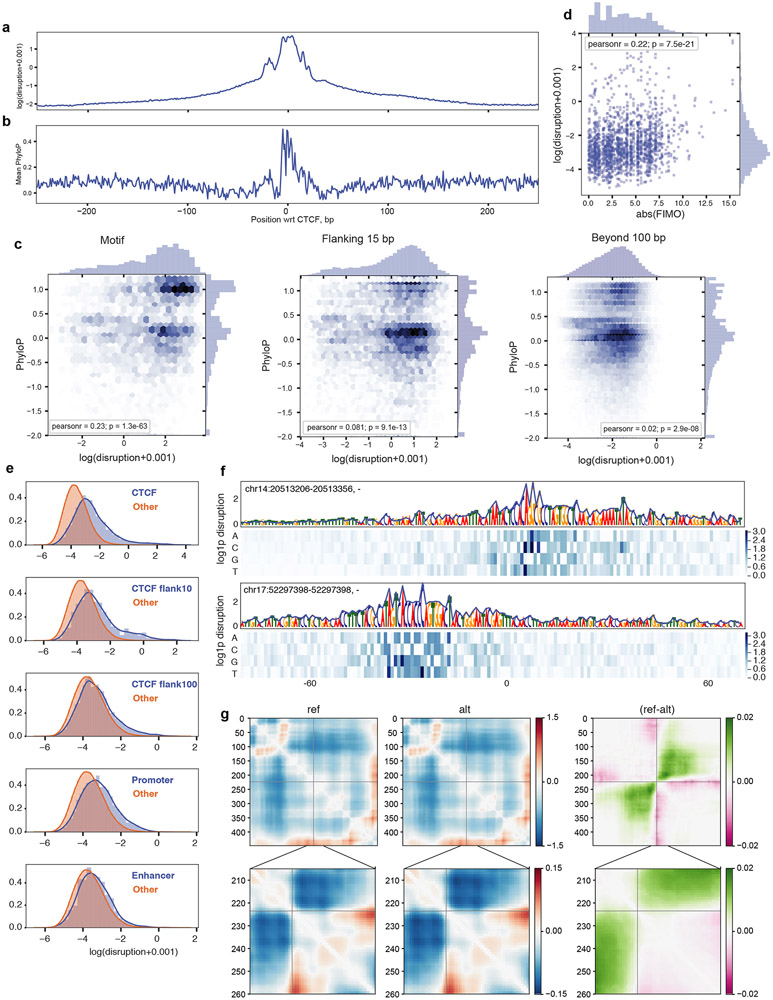
a-c. Predicted nucleotide-level impacts correlate with evolutionary conservation in and around CTCF motifs. Results from saturation mutagenesis of 500 bp regions around 500 randomly selected strong CTCF motifs, annotated by JASPAR with p-value < 1e-6, as for Fig. 3D. For each mutation, we computed the disruption score as the L2 norm of the predicted contact difference maps between the reference and alternative alleles. We aggregated scores across the model outputs by taking the mean. For visualization, these figures include a 0.001 pseudocount before taking the natural logarithm. We constructed a single score for each position by taking the maximum across alternative alleles.
a. The mean log disruption across regions is greatest within CTCF motifs, but is also high in the flanking regions.
b. The mean PhyloP score across regions is greatest within CTCF motifs, with peaks in similar places to nucleotide-level disruption scores. PhyloP values were extracted from the mammalian 30-way alignment for the same regions as in (a).
c. Scatter plots for disruption versus PhyloP scores for n=5,220 sites within CTCF motifs (top), n=7,830 sites in the flanking 15bp (middle), and n=73,341 sites beyond 100bp (bottom). We observed significant Pearson correlations within the CTCF motifs (top) and in the directly flanking regions (center), which drops off farther away (bottom).
d. Scatter plot for log disruption versus motif strength, computed as the absolute change of the FIMO score, for n=1,817 mutations that showed some evidence of influencing the CTCF motif. The wide range in Akita scores for a given change in FIMO score argues that Akita integrates nucleotide influences on genome folding beyond those described by a position weight matrix approach.
e-f. Large-scale mutagenesis reveals impactful annotation categories for single nucleotide variants. To quantify the impact of nucleotides within and near CTCF motifs relative to other genomic features we formed a set of unbiased mutations across the genome. We randomly selected 100,000 positions striding by 256 bp within the test set genomic regions and then selecting a random alternative nucleotide. For each mutation, we computed the disruption score as the L2 norm of the predicted contact difference maps between the reference and alternative allele, averaging across outputs.
e. Distributions of nucleotide disruption scores split by annotation category, compared to nucleotides outside of these annotation categories. We observed elevated scores in CTCF motifs, their flanking regions (CTCF Flank 10, CTCF Flank 100), promoters (500bp from GENCODE-annotated transcription start site), and enhancers (FANTOM5-annotated). For visualization we added a 0.001 pseudocount before taking the natural logarithm.
f. Two example sites without an annotation category. For visualization we added a 1 pseudocount before taking the natural logarithm (log1p). This suggests there are important DNA sequences for genome folding that remain uncharacterized.
g. Predicted maps for a high-scoring non-CTCF GTEx variant. Predicted maps underlying the score for chr7_5898574_G_T_b38 shown in Fig. 4g. Left: prediction for the reference allele. Middle: prediction for the alternative allele. Right: prediction for the (reference - alternate), where green indicates higher predicted contact frequency for the reference allele and pink indicates higher predicted contact frequency for the alternate allele. Top row: full prediction region. Bottom row: zoom into the boundary modified by the variant. Note the different color scales. Grey lines show the position of the variant, at the center of the prediction region. Akita predicts this variant modifies the strength of a nearby boundary. While difficult to see the influence of this single nucleotide change over the full prediction region, the difference becomes apparent upon subtraction of predicted maps. Specifically, this change indicates stronger predicted insulation at this boundary for the alternate allele (exp(0.02) ~= 2% decrease in contact frequency over this boundary).
Extended Data Fig. 8. Model predicts a redundant boundary at Lmo2.
Left: Predicted genome folding for unperturbed Lmo2 locus above the CTCF ChIP-seq profile for the region. Predictions in this figure used hg19 sequence as input and Akita’s output for HFF Micro-C.
Right: Numbers above maps indicate the (start,end) position of bins that were deleted, highlighted by purple shading on the zoomed-in CTCF ChIP-seq profile below the predicted WT map.
Akita predicts that deleting bins encompassing individual CTCF peaks (top row) would only mildly alter genome folding, and deletion of all three (bottom right) would be more impactful than either pair (bottom left and middle).
Extended Data Fig. 9. Cross-species predictions reveal impact of B2 SINE elements on genome folding in mouse embryonic stem cells.
a. MSE versus Spearman R for mouse regions that overlap regions syntenic to the human test set (mm10-syn-test, n=156 regions). MSE and Spearman R are both calculated per region for every (target, prediction) pair. Target Hi-C data was acquired from mouse embryonic stem cells31, mapped to mm10 and processed similarly to the previous human datasets. Predictions in this figure were made using mm10 sequence as input and Akita’s output for the H1hESC Micro-C dataset.
b. (left) Signal strength of predictions versus targets, for mm10-syn-test, calculated as the mean squared values in each map (same 156 regions shown as above). The model trained on human data shows an overall shift towards overly salient predictions in mouse relative to its predictions for human data (see Extended Data Fig. 3a for comparison). Black line shows x=y for reference here and below. (right) Squared error between targets and predictions correlates with the number of B2 SINE elements in the region (from RepeatMasker42).
c. Masking B2 SINE elements in input DNA sequences improved MSE for 93/156 predictions (~60%, left), and Spearman R for 106/156 predictions (~67%, right). This suggests that the mouse genome has evolved ways to mitigate the impact of its numerous B2 SINE elements on genome folding, which is supported by recent studies33.
d, e. Examples of improved predictions for two regions from the mm10-syn-test set after masking B2 SINEs, with the total number of B2 SINE elements per bin in the region displayed below each map. Initial predictions indicated in (a) with orange and green dots.
d. chr5:106334208-107382784 (deltaCorr:0.26, corrMutB2:0.72). Rectangle highlights a feature that is incorrectly predicted to be absent prior to masking B2 SINEs, and is correctly predicted following masking B2 SINEs.
e. chr14:61751296-62799872 (deltaCorr:0.18, corrMutB2:0.69). Rectangle highlights a feature that is incorrectly predicted to be present prior to masking B2 SINEs, and is correctly predicted following masking B2 SINEs.
Extended Data Fig. 10. A model trained with mouse genomic data correctly learns the minimal influence of B2 SINE sequences on genome folding.
a. MSE vs. Spearman R for a mm10-trained model on mm10 data (blue, n=384 regions shown), and the hg38-trained model on mm10 data (orange, n=156 regions shown). Each point represents a region from their respective test sets. The mm10 model was trained using Hi-C data from Bonev et al.31 (mESC, CN, ncx_CN, NPC, ncx_NPC) and Micro-C from Hsieh et al.43 (mESC) with the same multi-task framework used to train our hg38 model.
b,c. For the mm10-trained model, masking B2 SINE elements worsened MSE for 243/384 (63%) and Spearman R for 254/384 (66%) regions. MSE and Spearman R are both calculated per region for every (target, prediction) pair, overall pixels in the upper triangular region of predicted maps (n=99681 pixels).
Together (a-c) indicate the mm10-trained model correctly learns that B2 SINE elements have little impact on local genome folding and mutagenizing these elements leads to slightly worse predictive performance, in contrast with the hg38-trained model (see Extended Data Fig. 9).
d. Predictions for the regions from Extended Data Fig. 9 using the mm10-trained model. Note that the region from chr5 overlaps the training set for the mm10-trained model and the region from chr14 overlaps the test set.
Supplementary Material
Acknowledgements
The authors thank Vikram Agarwal, Han Yuan, and Elphege Nora for feedback on the manuscript. The authors thank Luis Chumpitaz-Diaz and Maureen Pittman for feedback on tutorials. The authors thank Nezar Abdennur and Peter Kerpedjiev for help with higlass visualization and Verena Heinrich for sharing mapped Capture-C reads. The authors thank Jacob Ulirsch, Qingbo Wang, and Hilary Finucane for sharing GTEx SuSiE fine mapping. GF and KSP were funded by Gladstone Institutes, the National Heart, Lung and Blood Institute (grant #HL098179), and the National Institute of Mental Health (grant #MH109907).
Footnotes
Competing interests
DRK is a paid employee of Calico Life Sciences, LLC.
References
- 1.Merkenschlager M & Nora EP CTCF and Cohesin in Genome Folding and Transcriptional Gene Regulation. Annu. Rev. Genomics Hum. Genet 17, 17–43 (2016). [DOI] [PubMed] [Google Scholar]
- 2.Krijger PHL & de Laat W Regulation of disease-associated gene expression in the 3D genome. Nat. Rev. Mol. Cell Biol 17, 771–782 (2016). [DOI] [PubMed] [Google Scholar]
- 3.Fudenberg G, Abdennur N, Imakaev M, Goloborodko A & Mirny LA Emerging Evidence of Chromosome Folding by Loop Extrusion. Cold Spring Harb. Symp. Quant. Biol 82, 45–55 (2017). [DOI] [PMC free article] [PubMed] [Google Scholar]
- 4.Rodríguez-Carballo E et al. The HoxD cluster is a dynamic and resilient TAD boundary controlling the segregation of antagonistic regulatory landscapes. Genes Dev. 31, 2264–2281 (2017). [DOI] [PMC free article] [PubMed] [Google Scholar]
- 5.Despang A et al. Functional dissection of the Sox9-Kcnj2 locus identifies nonessential and instructive roles of TAD architecture. Nat. Genet 51, 1263–1271 (2019). [DOI] [PubMed] [Google Scholar]
- 6.Cao F, Zhang Y, Loh YP, Cai Y & Fullwood MJ Predicting chromatin interactions between open chromatin regions from DNA sequences. bioRxiv 720748 (2019) doi: 10.1101/720748. [DOI] [Google Scholar]
- 7.Belokopytova PS, Nuriddinov MA, Mozheiko EA, Fishman D & Fishman V Quantitative prediction of enhancer-promoter interactions. Genome Res. 30, 72–84 (2020). [DOI] [PMC free article] [PubMed] [Google Scholar]
- 8.Zhang S, Chasman D, Knaack S & Roy S In silico prediction of high-resolution Hi-C interaction matrices. Nat. Commun 10, 5449 (2019). [DOI] [PMC free article] [PubMed] [Google Scholar]
- 9.Li W, Wong WH & Jiang R DeepTACT: predicting 3D chromatin contacts via bootstrapping deep learning. Nucleic Acids Res. 47, e60 (2019). [DOI] [PMC free article] [PubMed] [Google Scholar]
- 10.Whalen S, Truty RM & Pollard KS Enhancer–promoter interactions are encoded by complex genomic signatures on looping chromatin. Nat. Genet 48, 488–496 (2016). [DOI] [PMC free article] [PubMed] [Google Scholar]
- 11.Trieu T, Martinez-Fundichely A & Khurana E DeepMILO: a deep learning approach to predict the impact of non-coding sequence variants on 3D chromatin structure. Genome Biol. 21, 79 (2020). [DOI] [PMC free article] [PubMed] [Google Scholar]
- 12.Forcato M et al. Comparison of computational methods for Hi-C data analysis. Nat. Methods 14, 679–685 (2017). [DOI] [PMC free article] [PubMed] [Google Scholar]
- 13.Alipanahi B, Delong A, Weirauch MT & Frey BJ Predicting the sequence specificities of DNA- and RNA-binding proteins by deep learning. Nat. Biotechnol 33, 831–838 (2015). [DOI] [PubMed] [Google Scholar]
- 14.Kelley DR, Snoek J & Rinn JL Basset: learning the regulatory code of the accessible genome with deep convolutional neural networks. Genome Res. 26, 990–999 (2016). [DOI] [PMC free article] [PubMed] [Google Scholar]
- 15.Zhou J & Troyanskaya OG Predicting effects of noncoding variants with deep learning-based sequence model. Nat. Methods 12, 931–934 (2015). [DOI] [PMC free article] [PubMed] [Google Scholar]
- 16.Koo PK, Anand P, Paul SB & Eddy SR Inferring Sequence-Structure Preferences of RNA-Binding Proteins with Convolutional Residual Networks. bioRxiv 418459 (2018) doi: 10.1101/418459. [DOI] [Google Scholar]
- 17.Shrikumar A, Greenside P, Shcherbina A & Kundaje A Not Just a Black Box: Learning Important Features Through Propagating Activation Differences. arXiv:1605. 01713 [cs] (2016). [Google Scholar]
- 18.Kelley DR et al. Sequential regulatory activity prediction across chromosomes with convolutional neural networks. Genome Res. 28, 739–750 (2018). [DOI] [PMC free article] [PubMed] [Google Scholar]
- 19.Kelley DR Cross-species regulatory sequence activity prediction. PLoS Comput. Biol 16, e1008050 (2020). [DOI] [PMC free article] [PubMed] [Google Scholar]
- 20.Imakaev M et al. Iterative correction of Hi-C data reveals hallmarks of chromosome organization. Nat. Methods 9, 999–1003 (2012). [DOI] [PMC free article] [PubMed] [Google Scholar]
- 21.Yang T et al. HiCRep: assessing the reproducibility of Hi-C data using a stratum-adjusted correlation coefficient. Genome Res. 27, 1939–1949 (2017). [DOI] [PMC free article] [PubMed] [Google Scholar]
- 22.Nora EP et al. Targeted Degradation of CTCF Decouples Local Insulation of Chromosome Domains from Genomic Compartmentalization. Cell 169, 930–944.e22 (2017). [DOI] [PMC free article] [PubMed] [Google Scholar]
- 23.Wutz G et al. Topologically associating domains and chromatin loops depend on cohesin and are regulated by CTCF, WAPL, and PDS5 proteins. EMBO J. 36, 3573–3599 (2017). [DOI] [PMC free article] [PubMed] [Google Scholar]
- 24.Khan A et al. JASPAR 2018: update of the open-access database of transcription factor binding profiles and its web framework. Nucleic Acids Res. 46, D260–D266 (2018). [DOI] [PMC free article] [PubMed] [Google Scholar]
- 25.Pollard KS, Hubisz MJ, Rosenbloom KR & Siepel A Detection of nonneutral substitution rates on mammalian phylogenies. Genome Res. 20, 110–121 (2010). [DOI] [PMC free article] [PubMed] [Google Scholar]
- 26.Grant CE, Bailey TL & Noble WS FIMO: scanning for occurrences of a given motif. Bioinformatics 27, 1017–1018 (2011). [DOI] [PMC free article] [PubMed] [Google Scholar]
- 27.Rhee HS & Pugh BF Comprehensive genome-wide protein-DNA interactions detected at single-nucleotide resolution. Cell 147, 1408–1419 (2011). [DOI] [PMC free article] [PubMed] [Google Scholar]
- 28.Nakahashi H et al. A Genome-wide Map of CTCF Multivalency Redefines the CTCF Code. CellReports 3, 1678–1689 (2013). [DOI] [PMC free article] [PubMed] [Google Scholar]
- 29.Hnisz D et al. Activation of proto-oncogenes by disruption of chromosome neighborhoods. Science 351, 1454–1458 (2016). [DOI] [PMC free article] [PubMed] [Google Scholar]
- 30.Dixon JR et al. Topological domains in mammalian genomes identified by analysis of chromatin interactions. Nature 485, 376–380 (2012). [DOI] [PMC free article] [PubMed] [Google Scholar]
- 31.Bonev B et al. Multiscale 3D Genome Rewiring during Mouse Neural Development. Cell 171, 557–572.e24 (2017). [DOI] [PMC free article] [PubMed] [Google Scholar]
- 32.Schmidt D et al. Waves of Retrotransposon Expansion Remodel Genome Organization and CTCF Binding in Multiple Mammalian Lineages. Cell 148, 335–348 (2012). [DOI] [PMC free article] [PubMed] [Google Scholar]
- 33.Kaaij LJT, Mohn F, van der Weide RH, de Wit E & Bühler M The ChAHP Complex Counteracts Chromatin Looping at CTCF Sites that Emerged from SINE Expansions in Mouse. Cell 178, 1437–1451.e14 (2019). [DOI] [PubMed] [Google Scholar]
- 34.Kraft K et al. Serial genomic inversions induce tissue-specific architectural stripes, gene misexpression and congenital malformations. Nat. Cell Biol 21, 305–310 (2019). [DOI] [PubMed] [Google Scholar]
- 35.Schwessinger R et al. DeepC: Predicting chromatin interactions using megabase scaled deep neural networks and transfer learning. bioRxiv 724005 (2019) doi: 10.1101/724005. [DOI] [Google Scholar]
- 36.Krietenstein N et al. Ultrastructural Details of Mammalian Chromosome Architecture. Mol. Cell (2020) doi: 10.1016/j.molcel.2020.03.003. [DOI] [PMC free article] [PubMed] [Google Scholar]
- 37.Davis CA et al. The Encyclopedia of DNA elements (ENCODE): data portal update. Nucleic Acids Res. 46, D794–D801 (2018). [DOI] [PMC free article] [PubMed] [Google Scholar]
- 38.Gupta S, Stamatoyannopoulos JA, Bailey TL & Noble WS Quantifying similarity between motifs. Genome Biol. 8, R24 (2007). [DOI] [PMC free article] [PubMed] [Google Scholar]
- 39.Fulco CP et al. Activity-by-contact model of enhancer-promoter regulation from thousands of CRISPR perturbations. Nat. Genet 51, 1664–1669 (2019). [DOI] [PMC free article] [PubMed] [Google Scholar]
- 40.Beagan JA et al. YY1 and CTCF orchestrate a 3D chromatin looping switch during early neural lineage commitment. Genome Res. 27, 1139–1152 (2017). [DOI] [PMC free article] [PubMed] [Google Scholar]
- 41.Weintraub AS et al. YY1 Is a Structural Regulator of Enhancer-Promoter Loops. Cell 171, 1573–1588.e28 (2017). [DOI] [PMC free article] [PubMed] [Google Scholar]
- 42.Smit AFA, Hubley R & Green P RepeatMasker Open-4.0. 2013--2015. (2015). [Google Scholar]
- 43.Hsieh T-HS et al. Resolving the 3D Landscape of Transcription-Linked Mammalian Chromatin Folding. Mol. Cell (2020) doi: 10.1016/j.molcel.2020.03.002. [DOI] [PMC free article] [PubMed] [Google Scholar]
- 44.Goloborodko A, Venev S, Abdennur N, azkalot & Di Tommaso P mirnylab/distiller-nf: v0.3.3 (2019). doi: 10.5281/zenodo.3350937. [DOI] [Google Scholar]
- 45.Abdennur N & Mirny L Cooler: scalable storage for Hi-C data and other genomically-labeled arrays. Bioinformatics (2019) doi: 10.1093/bioinformatics/btz540. [DOI] [PMC free article] [PubMed] [Google Scholar]
- 46.Rao SSP et al. A 3D map of the human genome at kilobase resolution reveals principles of chromatin looping. Cell 159, 1665–1680 (2014). [DOI] [PMC free article] [PubMed] [Google Scholar]
- 47.Rao SSP et al. Cohesin Loss Eliminates All Loop Domains. Cell 171, 305–320.e24 (2017). [DOI] [PMC free article] [PubMed] [Google Scholar]
- 48.Wang S, Sun S, Li Z, Zhang R & Xu J Accurate De Novo Prediction of Protein Contact Map by Ultra-Deep Learning Model. PLoS Comput. Biol 13, e1005324 (2017). [DOI] [PMC free article] [PubMed] [Google Scholar]
- 49.Abadi M et al. TensorFlow. (2015). [Google Scholar]
- 50.Chollet F & Others. Keras. (GitHub, 2015). [Google Scholar]
- 51.Kandasamy K et al. Tuning Hyperparameters without Grad Students: Scalable and Robust Bayesian Optimisation with Dragonfly. arXiv [stat.ML] (2019). [Google Scholar]
- 52.Quinlan AR & Hall IM BEDTools: a flexible suite of utilities for comparing genomic features. Bioinformatics 26, 841–842 (2010). [DOI] [PMC free article] [PubMed] [Google Scholar]
- 53.Flyamer I et al. Phlya/adjustText: Trying zenodo. (2018). doi: 10.5281/zenodo.1494343. [DOI] [Google Scholar]
- 54.Aguet F et al. The GTEx Consortium atlas of genetic regulatory effects across human tissues. bioRxiv 787903 (2019) doi: 10.1101/787903. [DOI] [PMC free article] [PubMed] [Google Scholar]
- 55.Wang G, Sarkar A, Carbonetto P & Stephens M A simple new approach to variable selection in regression, with application to genetic fine-mapping. bioRxiv 501114 (2019) doi: 10.1101/501114. [DOI] [PMC free article] [PubMed] [Google Scholar]
- 56.Virtanen P et al. SciPy 1.0: fundamental algorithms for scientific computing in Python. Nat. Methods 17, 261–272 (2020). [DOI] [PMC free article] [PubMed] [Google Scholar]
- 57.van der Walt S, Colbert SC & Varoquaux G The NumPy Array: A Structure for Efficient Numerical Computation. Computing in Science Engineering 13, 22–30 (2011). [Google Scholar]
- 58.Reback J et al. pandas-dev/pandas: Pandas 1.0.3 (2020). doi: 10.5281/zenodo.3715232. [DOI] [Google Scholar]
- 59.Perez F & Granger BE IPython: A System for Interactive Scientific Computing. Computing in Science Engineering 9, 21–29 (2007). [Google Scholar]
- 60.Hunter JD Matplotlib: A 2D Graphics Environment. Computing in Science Engineering 9, 90–95 (2007). [Google Scholar]
- 61.Waskom M et al. seaborn: v0.5.0 (November 2014). (2014). doi: 10.5281/zenodo.12710. [DOI] [Google Scholar]
Associated Data
This section collects any data citations, data availability statements, or supplementary materials included in this article.
Supplementary Materials
Data Availability Statement
Datasets analysed in this study are publicly-available from: GEO (www.ncbi.nlm.nih.gov/geo/, Hi-C: GSE63525, GSE104334, GSE96107, 5C: GSE77142, Capture-C: GSE116794), 4D Nucleome Data Portal (https://data.4dnucleome.org/, Micro-C: 4DNESWST3UBH, 4DNES14CNC1I), UCSC (http://hgdownload.cse.ucsc.edu/goldenpath/hg38/database/), ENCODE data portal (www.encodeproject.org/), JASPAR (http://expdata.cmmt.ubc.ca/JASPAR/downloads/UCSC_tracks/2018/hg38/tsv/), GENCODE (https://www.gencodegenes.org/human/), FANTOM5 (https://fantom.gsc.riken.jp/data/).


