Abstract
Summary: Tag sequencing using high-throughput sequencing technologies are now regularly employed to identify specific sequence features, such as transcription factor binding sites (ChIP-seq) or regions of open chromatin (DNase-seq). To intuitively summarize and display individual sequence data as an accurate and interpretable signal, we developed F-Seq, a software package that generates a continuous tag sequence density estimation allowing identification of biologically meaningful sites whose output can be displayed directly in the UCSC Genome Browser.
Availability: The software is written in the Java language and is available on all major computing platforms for download at http://www.genome.duke.edu/labs/furey/software/fseq.
Contact: terry.furey@duke.edu
1 INTRODUCTION
High-throughput sequencing technologies that generate short sequence reads can be used to identify specific genomic features, such as transcription factor binding sites (Johnson et al., 2007; Robertson et al., 2007) and regions of open chromatin (Boyle et al., 2008) at a genome-wide level. In general, locations of biologically relevant features are defined by the presence of an enrichment of mapped sequence reads. To date, there is no standard means to summarize and visually display these data in an intuitive way. As the use of high-throughput sequencing becomes more prevalent, there is a growing need for a method to efficiently identify statistically significant genomic features based on sequence tags.
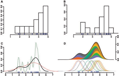
Published research using high-throughput sequencing data have employed histograms to calculate regions of dense sequence reads and make calls on sites of interest (Johnson et al., 2007; Robertson et al., 2007). Histograms are a non-parametric density estimator where the region covered is divided into equal-sized bins whose height is represented by the count of hits within that bin. These methods can be problematic as histograms are not smooth and can be strongly affected by the start/end points of the bins and the width of the bins (Fig. 1A and B).
Fig. 1.
Examples of histogram and density estimation properties. Blue dots represent sample positions being analyzed. (A, B) Locations of the bins used in histograms can cause data to look unimodal (A) or bimodal (B) depending on their starting positions (1.5 and 1.75, respectively). (C) Bandwidth affects the density generated in the same way as changing the size of bins. Over (red, dashed line) and under (green, dotted line) smoothed data can obscure the actual signal (black, solid line). (D) Example of how distributions over each point are combined to create the final distribution. Each of the samples are represented by Gaussian distributions which are summed to create the final density estimation.
To counteract bin boundary effects, one can instead calculate a kernel density estimate centered at each sequence allowing these estimates to overlap (Fig. 1D) (Parzen, 1962). Using a smooth kernel such as a Gaussian generates a smooth signal. This method does not alleviate the problem of bin width (or in the case of kernel density estimation, bandwidth) (Fig. 1C). Determination of an optimal bandwidth can present a problem, but this can be overcome by using the argument that minimizes the asymptotic mean integrated squared error (or other minimization techniques). However, the sparsity of data and size of whole-genomic sequences does not allow for estimating bandwidth with this method. Therefore, we suggest the use of a bandwidth based on the size of the feature being identified.
Although histogram methods have provided usable results, the dependency of resolution on bin size and the lack of statistical rigor in the treatment of the data begs for a new approach. We have developed an algorithm that uses kernel density estimation that can provide both a discrete and continuous probability landscape to better display genomic features of interest across the genome. These kernel density estimation-based probabilities, calculated at each base, are directly proportional to the probability of seeing a sequence read at that location.
2 F-SEQ DENSITY ESTIMATION
To generate the kernel density estimation, we consider the problem where we are given n sample points along a chromosome of length L. Our goal is to locate regions with high sample density. If we assume the points {xi}i=1n are sampled as  , then an estimate of this probability density function (pdf) will provide a significance measure for high density regions. We use the univariate kernel density estimation (kde) to infer the pdf, written as
| (1) |
where b is a bandwidth parameter controlling the smoothness of the density estimates, and K() is a Gaussian kernel function with mean 0 and variance 1. Instead of explicitly setting b, a user provides a feature length parameter (default=600) which controls the sharpness of the pdf estimate. Larger features will naturally lead to smoother density estimates.
Computing the density at each point in the chromosome using all n points is computationally expensive and exceeds the precision available to common computing platforms. We therefore compute a default window size w as a function of the bandwidth parameter b and the Gaussian kernel such that
We expect that window sizes for typical bandwidth settings will be on the order of a few thousand, significantly less than the many millions of bases available.
We also compute a threshold level for evaluating the significance of density regions using the following background model:
Compute an average number of features for window w as nw=nw/L.
Calculate the kernel density at a fixed point, xc, within the window given a random and uniform distribution of the nw features.
Repeat step 2 k times to obtain a distribution of the kernel density estimates for xc. For large k the kdes become normally distributed.
The threshold is s SDs above the mean of this normal distribution.
Larger values of s reduce the false discovery rate and provide a natural statistical interpretation to the veracity of these density regions.
F-Seq takes an input a BED format file (http://genome.ucsc.edu/FAQ/FAQformat#format1) containing aligned sequence tags. Since calculation of kernel density estimation requires a point measure for each sequence, we use the estimated center of the DNA fragment being sequenced. In many cases, such as from ChIP-seq protocols, the aligned sequence represents only the 5′ end of a longer fragment and therefore should be extended to the average fragment size in the experiment. In the case of DNase-Seq protocols where the 5′ end of the sequence represents the point of enrichment, the alignment should be shortened to 1 bp in length. A perl script has been included to perform this task.
Output files can be created either as a continuous probability wiggle format (http://genome.ucsc.edu/goldenPath/help/wiggle.html) or as a discrete-scored regions BED format. The discrete regions are those where the continuous probability is above the threshold s SDs above the background mean. These output files are ready for immediate import into the UCSC Genome Browser (Kent et al., 2002) (http://genome.ucsc.edu).
3 EXAMPLE APPLICATIONS
3.1 DNase I hypersensitive sites (DNase-seq)
To demonstrate that our algorithm can perform at or above previously demonstrated methods, we applied it to high-throughput data from DNase I hypersensitive sites (Boyle et al., 2008). This set consisted of 12 619 784 uniquely aligned sequences that should be over-represented at hypersensitive sites. To compare F-Seq with window-based clustering methods, we used a set of 287 DNaseI HS sites and 321 DNaseI-resistant sites. This set of data showed that F-Seq outperformed window clustering with an area under the receiver operator characteristic (ROC) curve of 0.946 versus 0.914.
3.2 Chromatin immunoprecipitation (ChIP-seq)
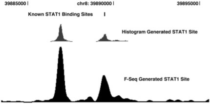
As most current applications of this technology are using chromatin immunoprecipitation samples for sequencing, we also wish to demonstrate the applicability of our algorithm to these data (Fig. 2). For our comparison we used 8 679 818 unique sequence reads from interferon-γ stimulated HeLa S3 cells (Robertson et al., 2007). Spearman correlation of our peaks with the peaks reported in the article was 0.917 and distance to the list of 28 known motifs which were identified using the windowing method was slightly improved (on average 2 bp closer). There is a broad range of peak sizes resulting from these experiments that may require different bandwidth settings. If warranted, multiple bandwidth settings may be used to elucidate both the large and fine structure of the data.
Fig. 2.
View of 10 kb region of Chromosome 8 shows an accurate duplication of windowing technique in STAT1 data (Robertson et al., 2007). Note that the histogram generated sites from Robertson et al. only display sites above a cutoff.
ACKNOWLEDGEMENTS
This material is based upon work supported under a National Science Foundation Graduate Research Fellowship.
Funding: This material is based upon work supported under a National Science Foundation Graduate Research Fellowship and NIH Grants HG004563 and HG003169.
Conflict of Interest: none declared.
REFERENCES
- Boyle AP, et al. High-resolution mapping and characterization of open chromatin across the genome. Cell. 2008;132:311–322. doi: 10.1016/j.cell.2007.12.014. [DOI] [PMC free article] [PubMed] [Google Scholar]
- Johnson DS, et al. Genome-wide mapping of in vivo protein-DNA interactions. Science. 2007;316:1497–1502. doi: 10.1126/science.1141319. [DOI] [PubMed] [Google Scholar]
- Kent WJ, et al. The human genome browser at UCSC. Genome Res. 2002;12:996–1006. doi: 10.1101/gr.229102. [DOI] [PMC free article] [PubMed] [Google Scholar]
- Parzen E. On the estimation of a probability density function and mode. Ann. Math. Stat. 1962;33:1065–1076. [Google Scholar]
- Robertson G, et al. Genome-wide profiles of STAT1 DNA association using chromatin immunoprecipitation and massively parallel sequencing. Nat. Methods. 2007;4:651–657. doi: 10.1038/nmeth1068. [DOI] [PubMed] [Google Scholar]


