

Abstract
Excitatory pyramidal neurons and inhibitory interneurons constitute the main elements of cortical circuitry and have distinctive morphologic and electrophysiological properties. Here, we differentiate them by analyzing the time course of their action potentials (APs) and characterizing their receptive field properties in auditory cortex. Pyramidal neurons have longer APs and discharge as regular-spiking units (RSUs), whereas basket and chandelier cells, which are inhibitory interneurons, have shorter APs and are fast-spiking units (FSUs). To compare these neuronal classes, we stimulated cat primary auditory cortex neurons with a dynamic moving ripple stimulus and constructed single-unit spectrotemporal receptive fields (STRFs) and their associated nonlinearities. FSUs had shorter latencies, broader spectral tuning, greater stimulus specificity, and higher temporal precision than RSUs. The STRF structure of FSUs was more separable, suggesting more independence between spectral and temporal processing regimens. The nonlinearities associated with the two cell classes were indicative of higher feature selectivity for FSUs. These global functional differences between RSUs and FSUs suggest fundamental distinctions between putative excitatory and inhibitory interneurons that shape auditory cortical processing.
Keywords: fast-spiking, regular-spiking, spectrotemporal, auditory cortex, interneuron, receptive field
Introduction
Sensory cortex contains both excitatory and inhibitory cells whose functional role in shaping local processing has not been fully determined (Fairén et al., 1984; Houser et al., 1984). These cells are fundamental components of neocortical circuits, providing both feedforward and recurrent connections in all modalities and species (Callaway, 1998, 2004; Douglas and Martin, 2004). Although both neuron types are found in the same circuit, their connection patterns, and thus their functional properties, likely differ (Thomson et al., 2002). A constraint on this connectional complexity is that excitatory neurons can have both long-range (>1 mm) and short-range connections, whereas inhibitory interneurons display more local connection patterns (Holmgren et al., 2003; Markram et al., 2004).
In the primary auditory cortex (AI), a diverse number of cell types have been identified based on morphology, neurotransmitter type, and connectivity (Winer, 1992). Excitatory cells comprise ∼75% of the neural population and are highly correlated with pyramidal cell morphology (Douglas and Martin, 2004). Inhibitory interneurons seem much more diverse because they may be classified according to different morphological, physiological, molecular, and synaptic properties (Kawaguchi, 1993a; Kawaguchi and Kubota, 1997; Markram et al., 2004). Recent studies promise to expand these classification schemes by analyzing cells based on gene expression, suggesting an even more diverse family of inhibitory interneurons (Wang et al., 2002; Toledo-Rodriguez et al., 2004; Wang et al., 2004; Sugino et al., 2006).
Inhibitory interneurons provide feedforward and feedback inhibition onto excitatory cells, although the role served by these contacts has not been fully delineated (Miller, 2003; Gabernet et al., 2005; Cruikshank et al., 2007; Silberberg and Markram, 2007). Little is known about the receptive field properties of AI inhibitory interneurons because it is challenging to anatomically identify and record from them (Mitani and Shimokouchi, 1985; Mitani et al., 1985). In primary visual cortex, inhibitory interneurons have simple or complex receptive field properties, resembling their excitatory counterparts (Azouz et al., 1997; Hirsch et al., 2003). In somatosensory cortex, inhibitory interneurons have larger receptive fields and higher firing rates than excitatory cells (Simons and Carvell, 1989; Bruno and Simons, 2002). In contrast, little progress has been made on delineating the receptive field structure of auditory cortical inhibitory interneurons and comparing it with excitatory cells (de Ribaupierre et al., 1972; Volkov et al., 1989). Inhibitory interneurons are most readily identified using intracellular labeling and reconstruction coupled with histochemical techniques. This anatomical evidence, however, is difficult to accrue in combination with extensive physiological characterization. Recent work has used the features of extracellular action potentials (APs) to distinguish two physiological types of cortical neurons, regular-spiking units (RSUs) and fast-spiking units (FSUs). RSUs, which correspond predominantly to pyramidal neurons, have longer APs, whereas FSUs typically have briefer APs both in vitro and in vivo, thus integrating anatomical and physiological results (McCormick et al., 1985; Bruno and Simons, 2002; Andermann et al., 2004; Barthó et al., 2004). FSUs often correlate with parvalbumin-stained cortical cells and thus correspond to basket and chandelier cells, which are inhibitory interneurons that are essential components in the AI microcircuit (Hendry and Jones, 1991; McMullen et al., 1994; Kawaguchi and Kubota, 1997).
We classified AI neurons based on their AP shape into RSUs or FSUs and computed their spectrotemporal receptive fields (STRFs) and the accompanying nonlinearities. This permitted functional comparisons between the different neuron types according to their selectivity for different spectrotemporal stimulus features.
Materials and Methods
The electrophysiological recording methods and stimulus design have been described in previous reports (Miller and Schreiner, 2000; Miller et al., 2001a,b, 2002). A brief description follows.
Electrophysiology.
All procedures were in compliance with the University of California, San Francisco Committee for Animal Research and the guidelines of the Society for Neuroscience and in compliance with National Institutes of Health guidelines (publication 85-23). Cats (Felis catus; female, 8–18 months of age; n = 8) were first given ketamine (22 mg/kg) and acepromazine (0.11 mg/kg) and then anesthetized with pentobarbital sodium (Nembutal, 15–30 mg/kg) for the surgical procedure. The animal's core temperature was maintained with a thermostatic heating pad. Bupivicaine was infiltrated into incisions and pressure points. A tracheotomy, reflection of the soft tissues of the scalp, craniotomy over AI, and durotomy were made. For the recording session, the animal was maintained in an areflexive state with a continuous infusion of ketamine/diazepam (2–10 mg · kg−1 · h−1 ketamine, 0.05–0.2 mg · kg−1 · h−1 diazepam in lactated Ringer's solution).
Recordings were made in a sound-shielded anechoic chamber (IAC, Bronx, NY), with stimuli delivered monaurally to the ear contralateral to the exposed cortex via a closed speaker system (diaphragms from Stax, Saitama, Japan). Simultaneous extracellular recordings were made using multichannel silicon recording probes provided by the University of Michigan Center for Neural Communication Technology (Wise, 2005). The probes contained 16 linearly spaced recording channels, each separated by 150 μm. The area of each electrode contact was 177 μm2, and the impedance of each channel was 2–3 MΩ. Probes were positioned orthogonally to the cortical surface and lowered to 2300–2400 μm using a microdrive (David Kopf Instruments, Tujunga, CA).
Neural traces were bandpass filtered between 600 and 6000 Hz and recorded to disk with a Neuralynx (Bozeman, MT) Cheetah analog-to-digital system at sampling rates between 18,000 and 27,000 Hz. Stimulus-driven neural activity was recorded for ∼75 min at each location. After each experiment, the traces were sorted off-line with a Bayesian spike-sorting algorithm (Lewicki, 1994). Each probe penetration yielded 8–16 active channels, with approximately one to two well isolated single units per channel. Only these well isolated units were used in receptive field analyses.
Stimulus.
Neurons were first probed with pure tones and then with one or two presentations of a 15 or 20 min dynamic moving ripple stimulus, followed by ∼20 min of silence, during which spontaneous activity was recorded. Each pure tone was presented five times. The level and frequency of each pure tone was chosen randomly from 15 different levels (5 dB sound pressure level spacing) and 45 different frequencies. The dynamic ripple stimulus is a temporally varying broadband sound (500–20,000 or 40,000 Hz) composed of ∼50 sinusoidal carriers per octave, each with randomized phase (Escabí and Schreiner, 2002). The carrier magnitude at any time is modulated by the spectrotemporal envelope, consisting of sinusoidal amplitude peaks (“ripples”) on a logarithmic frequency axis that changes through time. Spectral and temporal modulation parameters define the stimulus envelope. Spectral modulation rate is characterized by the number of spectral peaks per octave. Temporal modulations are defined by the speed and direction of the changes of the peaks. The spectral and temporal modulation parameters varied randomly and independently during the stimulus. Spectral modulation rate varied slowly (maximum rate of change, 1 Hz) between 0 and 4 cycles per octave; the temporal modulation rate varied between −40 Hz (upward sweep) and 40 Hz (downward sweep), with a maximum 3 Hz rate of change. Maximum modulation depth of the spectrotemporal envelope was 40 dB. Mean intensity was set 30–50 dB above the pure-tone threshold of the neuron.
Analysis.
Data analysis was performed in Matlab (MathWorks, Natick, MA). For each neuron, frequency response areas were computed from the pure-tone responses, whereas the reverse correlation method was used to derive the STRF, which is the average spectrotemporal stimulus envelope preceding each spike (Aertsen and Johannesma, 1980; deCharms et al., 1998; Klein et al., 2000; Theunissen et al., 2000; Escabí and Schreiner, 2002). Positive regions of the STRF indicate that stimulus energy at that frequency and time will increase the firing rate of the neuron above the average rate, and negative regions indicate the converse.
Characterization of the temporal and spectral modulation properties were derived by computing a two-dimensional fast Fourier transform (2D FFT) of each significant STRF and then folding the absolute value of the 2D FFT along the temporal modulation frequency axis, to obtain the ripple transfer function (RTF). Because the Fourier transform is sensitive to periodicities in the STRF envelope, the RTF reflects the relationship of excitatory and suppressive STRF subfields.
Temporal (tMTF) and spectral (sMTF) modulation transfer functions were obtained by summing the RTF along the spectral and temporal modulation axis, respectively. MTFs were classified as bandpass if, after identifying the peak in the MTF, values at lower and higher modulation rates decreased by at least 3 dB. If there was no such decrease, the MTF was classified as low pass. High-pass MTFs were not encountered. Best modulation rate for bandpass MTFs corresponded to the peak value in the MTF, whereas for low-pass MTFs, it was the mean between the 0 modulation frequency value and the 3 dB high-side cutoff. MTF width for bandpass MTFs was the difference between the high and low modulation rate 3 dB cutoff values, whereas for low-pass MTFs, the width was the difference between the high-side 3 dB cutoff rate and the 0 modulation frequency value.
The inseparability of the STRF was determined by performing singular value decomposition (Depireux et al., 2001). The inseparability index (ISPI) was defined as
where σ1 is the largest singular value. The ISPI, which ranges between 0 and 1, describes how well the STRF may be described by a pair of one-dimensional functions: one a function of time and the other a function of frequency, with values near 0 corresponding to an STRF for which time and frequency may be dissociated.
Using previously described methodologies, we computed a phase-locking index (PLI) for each neuron using the relation ), where max(STRF) and min(STRF) are the maximum and minimum values in the STRF, and r is the average firing rate (Escabí and Schreiner, 2002). The square root of 8 allows the PLI to range from 0 (not phase locked) to 1 (precisely phase locked).
To determine the stimulus selectivity of each neuron, we calculated a feature selectivity index (FSI) for each neuron (Miller et al., 2001a; Escabí and Schreiner, 2002). For each spike generated by the neuron, the ripple envelope that preceded the spike was captured and correlated with the STRF of the neuron. The similarity index (SI) is formally defined as follows:
 |
where stim and STRF are matrices that represent the stimulus segment preceding a spike and the receptive field of the neuron, respectively, and i and j range over the number of rows and columns in the STRF. The SI ranges between −1 and +1 and is a measure of the spectrotemporal correlation between the stimulus and the STRF.
A similarity index value was calculated for each action potential, forming an SI probability distribution, P(SI), of the driven activity. Using a spike train of similar length but from random spikes (Miller et al., 2001a, 2002), we calculated SIs from the STRF of the neuron and formed a probability distribution, Prand(SI), for a random selection of stimulus segments. For each SI probability distribution, the cumulative distribution function (CDF) was then calculated according to the following:
The difference between the random and driven spike trains was quantified by obtaining the areas, A and Arand, under each cumulative distribution function, from which we then calculated the FSI as follows:
FSI values vary between 0 and 1, where 0 corresponds to similar distributions for Prand(SI) and P(SI), i.e., a neuron that responds indiscriminately to stimulus segments, and 1 corresponds to a neuron that is responsive to a very restricted range of stimulus features.
For each STRF, we computed the nonlinear function that related the stimulus to the probability of spike occurrence. Each ripple stimulus segment, s, that elicited a spike was correlated with the STRF by projecting it onto the STRF via the inner product z = s × STRF. The projection, or stimulus-filter similarity, characterizes the probability distribution P(z|spike). We then projected a large number of randomly selected stimulus segments onto the STRF and formed the prior stimulus distribution, P(z). The projection values that comprised P(z|spike) and P(z) were transformed to units of SD by normalizing relative to the mean, μ, and SD, σ, of P(z), using x = (z − μ)/σ. The nonlinearity for the STRF was then computed as
where P(spike) is the average firing rate of the neuron (Aguera y Arcas et al., 2003). Thus, the nonlinearity describes the likelihood of a spike occurrence given the similarity between the STRF and the stimulus. The FSI and the integral of P(x|spike) are closely related measures.
Results
We recorded STRFs from 1252 single neurons across all cortical layers in cat AI and classified 1093 neurons as either RSUs or FSUs. To distinguish FSUs from RSUs, we characterized the action potential waveforms of the recorded neurons using previously proposed criteria (Bruno and Simons, 2002; Barthó et al., 2004). Two representative action potentials, with example traces from which the action potential shapes were inferred, are shown in Figure 1A. Each action potential was analyzed, and the phases of the action potential were quantified (Fig. 1B). The dotted lines indicate different temporal phases of the waveform that were used for classification purposes.
Figure 1.
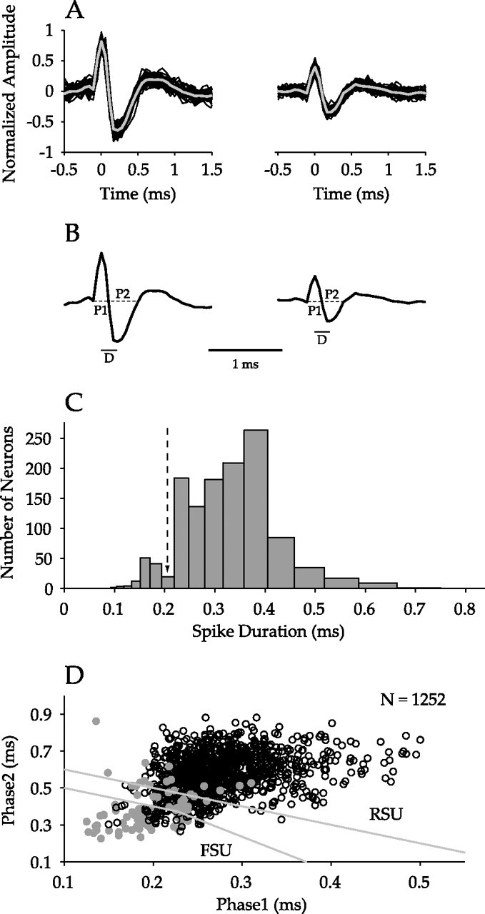
Classification of AI neurons. A, Two single neurons recorded from the same channel of the multichannel probe. Shown are 50 representative traces (black), with the derived action potential waveform template superimposed (gray). B, Analysis of action potential shape. P1 and P2 denote phase 1 and phase 2, the durations of the two segments of the waveform. D represents the time between the peak and the trough in the waveform. C, Histogram of time between peak and trough in the waveform across all neurons (n = 1252). The dashed arrow at ∼0.2 ms represents the FSU/RSU classification boundary from the study by Mitchell et al. (2007). D, Separation of FSUs and RSUs following the study by Bruno and Simons (2002). By plotting phase 2 against phase 1, FSUs (n = 115) are classified as those neurons falling below the lower gray lines. RSUs (n = 978) are signified by points above the top gray line. Filled gray circles represent neurons for which D ≤ 0.2 ms.
The action potential duration was calculated as the time between the waveform maximum and minimum values (Fig. 1C) (Mitchell et al., 2007). In the histogram, a mode is present for values <0.2 ms, in accord with a previously used boundary between FSUs and RSUs (Mitchell et al., 2007). FSUs and RSUs may also be classified based on the action potential temporal phases (Fig. 1D). Here, all recorded neurons are shown, with cells that also had action potential durations <0.2 ms marked in gray. Unlike reports in barrel cortex (Bruno and Simons, 2002; Andermann et al., 2004), the phase plot does not show two distinct clusters with a clear classification boundary but reveals a continuum for the relationship between the two temporal phases. This could reflect the larger sample size or it could be a consequence of the overall faster kinetics of AI neurons (Hefti and Smith, 2003).
All neurons, including those that had action potential durations <0.2 ms, had to satisfy two criteria to be classified as FSUs. First, the sum of the two temporal phases, phase 1 and phase 2, had to be <0.6 ms. Second, a classification boundary was chosen from a previous report, in which clear separation was seen between FSUs and RSUs (Bruno and Simons, 2002) and was calculated to be (1.8824 × phase 1 + phase 2 = 0.8). A total of 115 neurons satisfied these constraints and were labeled FSUs. Neurons with (phase 1 + phase 2 > 0.7 ms) were classified as RSUs (n = 978). To reduce the probability of classification error, neurons with phase 1 and phase 2 sums >0.6 ms and <0.7 ms (n = 159) were excluded from additional analysis.
Because multichannel probes were used, the cortical depth of each neuron could be defined. Most neurons (778 of 1252) resided between 600 and 1600 μm, although recordings included the full cortical width. We found FSUs at all depths, with population peaks at 800–1000 μm and at 1400–1600 μm, corresponding to layer 4, and deep layer 5 and superficial layer 6 (Fig. 2A), indicating that FSUs are concentrated in different AI laminae. The distribution of RSUs was more uniform across the depth of AI (Fig. 2B). The ratio of the number of FSUs to RSUs at different depths also revealed the two FSU peaks, as well as one at the most superficial depths of cortex (Fig. 2C). The FSU profile peaks are consistent with anatomical studies in cat and rabbit AI that indicated two local peaks, in layer 4 and layer 6, for parvalbumin-stained neurons (Hendry and Jones, 1991; McMullen et al., 1994). FSUs most often correspond to basket and chandelier cells, which stain positively for parvalbumin, thus lending support for the FSU/RSU classification approach used in this study (Kawaguchi, 1993a; Kawaguchi and Kondo, 2002).
Figure 2.
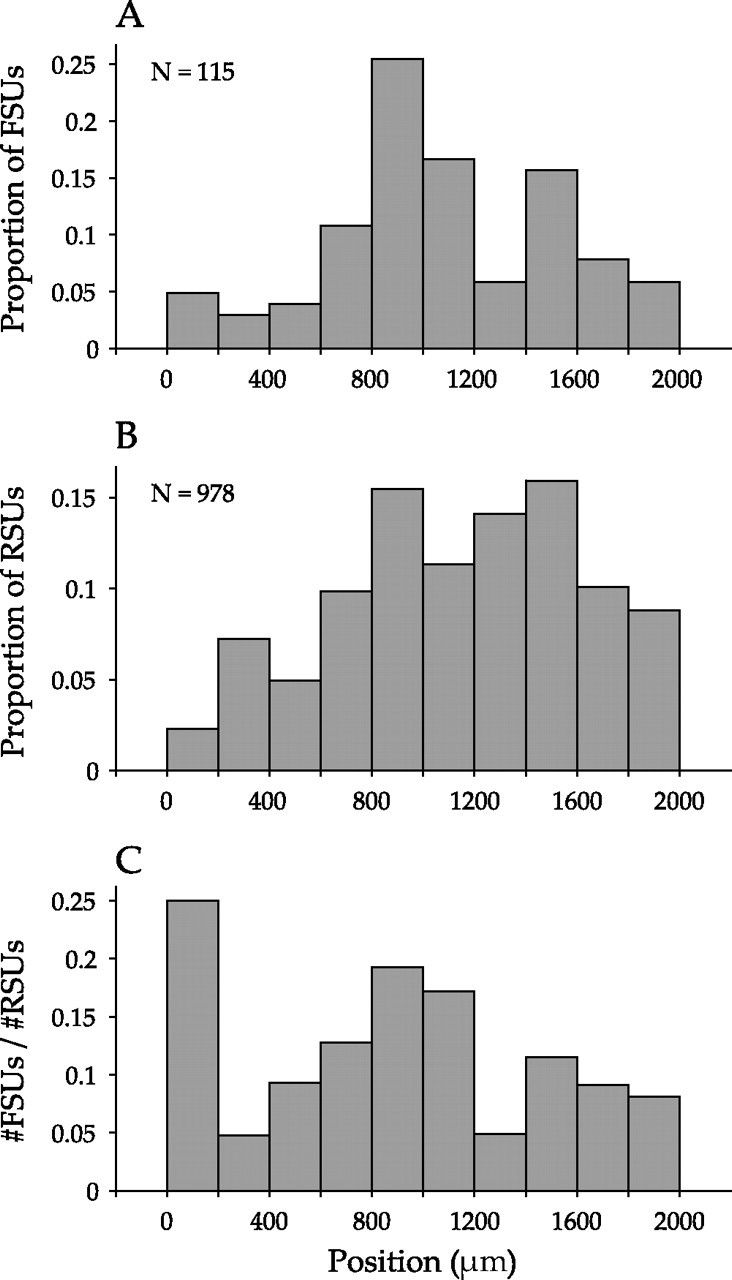
Depth distribution of recorded AI neurons. A, Distribution of recording depths for FSUs. The abscissa indicates recording position below the cortical surface, whereas the ordinate describes the proportion of the recorded FSU population (n = 115). Two peaks are present from 800–1200 and 1400–1600 μm. B, Distribution of RSUs (n = 978). C, Depth distribution for the ratio of the number of identified FSUs to RSUs. Two FSU peaks are present, as well as an additional peak at 0–200 μm.
The following sections compare functional properties of FSUs and RSUs. A summary of the differences or similarities for each of the analyzed parameters is given in Table 1.
Table 1.
Comparison of FSU and RSU receptive field parameters
| Parameter | FSU | Comparison | RSU |
|---|---|---|---|
| Characteristic frequency range (kHz) | 6.9–25.6 | = | 6.1–26.4 |
| Latency (ms) | 11.6 (3.4) | < | 13.2 (4.3) |
| Sharpness of tuning (Q) | 3.5 (1.3) | < | 3.9 (1.3) |
| Firing rate (sp/s) | 5.9 (7.9) | < | 6.7 (7.2) |
| Phase locking index | 0.19 (0.14) | > | 0.11 (0.09) |
| Temporal BMF (cycles/s) | 14.1 (6.2) | = | 13.0 (5.3) |
| Spectral BMF (cycles/octave) | 0.89 (0.46) | = | 0.97 (0.51) |
| % Bandpass tMTFs | 65 | > | 47 |
| % Bandpass sMTFs | 25 | > | 15 |
| Inseparability index | 0.36 (0.18) | < | 0.44 (0.18) |
| Feature selectivity index | 0.14 (0.10) | > | 0.09 (0.07) |
| Nonlinearity skewness | 1.72 (0.68) | > | 1.52 (0.71) |
| % Monotonic nonlinearities | 70 | = | 64 |
| Nonlinearity asymmetry index | 0.84 (0.17) | > | 0.76 (0.17) |
Values are population means, with SDs in parentheses. The third column indicates whether the FSU/RSU parameters were statistically different (p < 0.05). < indicates the FSU parameter was significantly less than the RSU parameter, > indicates significantly greater, and = indicates no significant difference (p > 0.05).
Basic receptive field parameters
Basic response properties of FSUs and RSUs were first compared using standard receptive field parameters. Frequency response characteristics were assessed by first extracting the characteristic frequency (CF) of each FSU from the STRF (Fig. 3A). Because each FSU was recorded using a multichannel probe, the mean of all RSU CFs from the same probe penetration was used as a comparison. This comparison was made for each individual FSU in a probe penetration. The FSU and RSU CF distributions were not significantly different (range, ∼6–25 kHz; p = 0.26, signed-rank test), with FSU and RSU CFs highly correlated (Fig. 3B) (r = 0.88; p < 0.01, t test), thus supporting a columnar organization of CF. The average CF difference between the mean for RSUs and for individual FSUs in a penetration was 0.12 ± 0.15 octaves. The same comparison procedure was followed for the sharpness of tuning (quality factor, Q: CF/bandwidth at 90% below excitatory peak) (Schreiner and Mendelson, 1990). Q values were significantly correlated for FSU/RSU data (Fig. 3C) (r = 0.57; p < 0.01). However, the distributions were significantly different, with FSUs more broadly tuned than RSUs (FSU mean/SD, 3.48/1.30; RSU mean/SD, 3.90/1.32; p < 0.01, signed-rank test). Peak excitatory response latency of the STRF for each FSU was also compared with that of RSUs. Here, the latency of the FSU was compared with the mean of the latencies of RSUs in the same layer and in the same penetration as the FSU, with the comparison made for each FSU in a given penetration. FSU and mean RSU latencies were significantly correlated (Fig. 3D) (r = 0.76; p < 0.01, t test) within each penetration, with FSUs having shorter latencies (FSU mean/SD, 11.6/3.4 ms; RSU mean/SD, 13.2/4.3 ms; p < 0.01, signed-rank test).
Figure 3.

Basic receptive field parameter analysis. A, Parameters obtained from STRFs. The STRF is the average stimulus preceding a spike, with the abscissa representing time before a spike and frequency on the ordinate. Red indicates time–frequency combinations that lead to an increase in firing rate, whereas blue represents a decrease. STRFs are scaled relative to their maximum value. From each STRF, CF, bandwidth (BW), Q values (Q = CF/BW), and the latency were obtained. B, Comparison of FSU and RSU CFs. FSUs and RSUs in the same penetration shared similar CFs. The diagonal line represents equality between the FSU and RSU values. C, Comparison of FSU and RSU sharpness of tuning. Q values were lower for FSUs, indicating that they are more broadly tuned than RSUs. D, Comparison of latencies. FSU latencies were shorter than those of RSUs.
A basic response characteristic of a neuron is its firing rate in response to a stimulus. To compare FSU and RSU response patterns, we plotted the distribution of firing rates over the course of the ripple stimulus.
FSUs are dominated by low firing rates for the ripple stimulus, mostly less than 3 spikes per second (sp/s) (Fig. 4A) (FSU median, 2.66 spikes per second), whereas RSUs show a clear exponential distribution of firing rates, consistent with previous experimental and theoretical work (Baddeley et al., 1997; Attwell and Laughlin, 2001; Lennie, 2003). The RSU firing rate distribution (Fig. 4B) decays smoothly from low to high rates (RSU median, 4.40 sp/s). The firing rate CDFs (Fig. 4C) separate at ∼3 sp/s and are significantly lower for FSUs [p < 0.01, Kolmogorov–Smirnov (KS) test].
Figure 4.
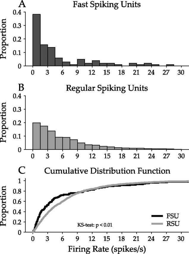
Comparison of firing rate for FSUs and RSUs. Firing rate was calculated from the response to one dynamic moving ripple stimulus presentation. A, FSU firing rate distribution. The highest proportion of FSUs have firing rates below 6 sp/s. B, The RSU firing rate distribution is approximately exponential, with the proportion of RSUs decaying from low to high firing rates. C, Cumulative distribution functions for FSU and RSU firing rates. The two distributions are significantly different, with FSUs having lower firing rates than RSUs (p < 0.01, KS test).
Although FSU firing rates were significantly lower, this may not affect the temporal precision of FSU responses. We computed a PLI for each neuron: if spikes were poorly synchronized to a particular stimulus phase, i.e., they show considerable temporal jitter, then the STRF peaks and troughs would be shallower, scaling with the average spike rate (Escabí and Schreiner, 2002).
FSUs and RSUs had significantly different degrees of phase locking (Fig. 5A,B). FSUs had higher PLIs and thus higher temporal precision in their relationship of spike occurrence and stimulus waveform (FSU mean/SD, 0.19/0.14; RSU mean/SD, 0.11/0.09). This difference is evident in the cumulative distribution function (Fig. 5C) (p < 0.01, KS test). The temporal jitter of RSU spikes was 65% larger than for FSUs. Thus, FSUs fire fewer spikes, although the generated spikes are aligned more precisely to specific ripple stimulus segments and thus represent a more accurate and reproducible temporal response pattern than RSUs.
Figure 5.
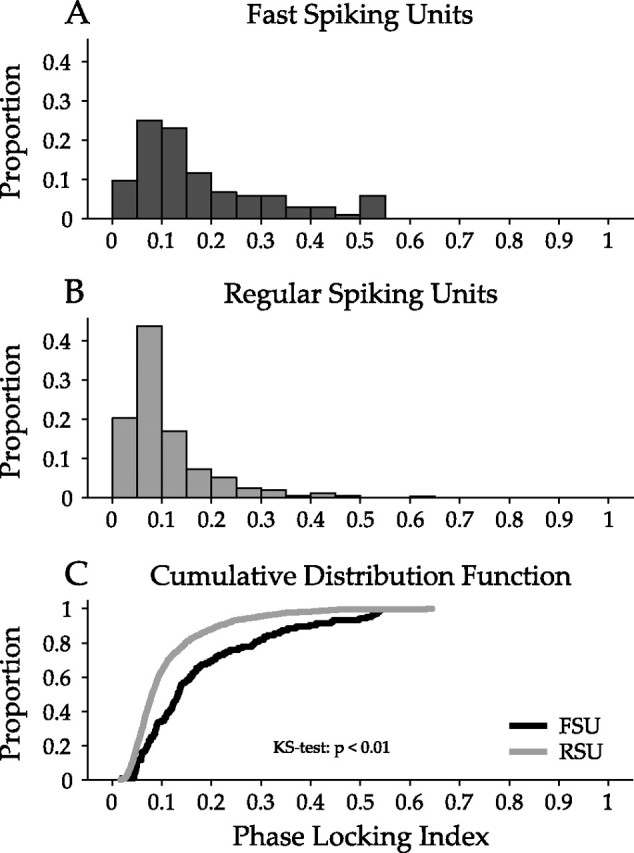
Analysis of the temporal precision of FSU and RSU responses. Comparison of phase locking to the ripple stimulus envelope for FSUs and RSUs. The phase-locking index quantifies how well the response is locked to specific temporal aspects of the ripple stimulus. Phase-locking values near 1 indicate precise temporal precision in the response, whereas those near 0 indicate little precision. A, FSU phase-locking distribution extends to 0.55. B, RSU phase-locking distribution extends to 0.3. C, Comparison of phase-locking cumulative distribution functions for FSUs and RSUs. FSUs responded with significantly better temporal precision than RSUs (p < 0.01, KS test).
Spectrotemporal receptive field parameters
STRF structure reflects a more complete picture of the spectrotemporal stimulus features that elicit a neuronal response than the properties considered thus far. The RTF for each neuron constitutes an equivalent way of characterizing these features and is computed from the 2D FFT of the STRF (Fig. 6A,B). The RTF has axes that represent the spectral and temporal modulation spectra captured by a neuron (Fig. 6C).
Figure 6.
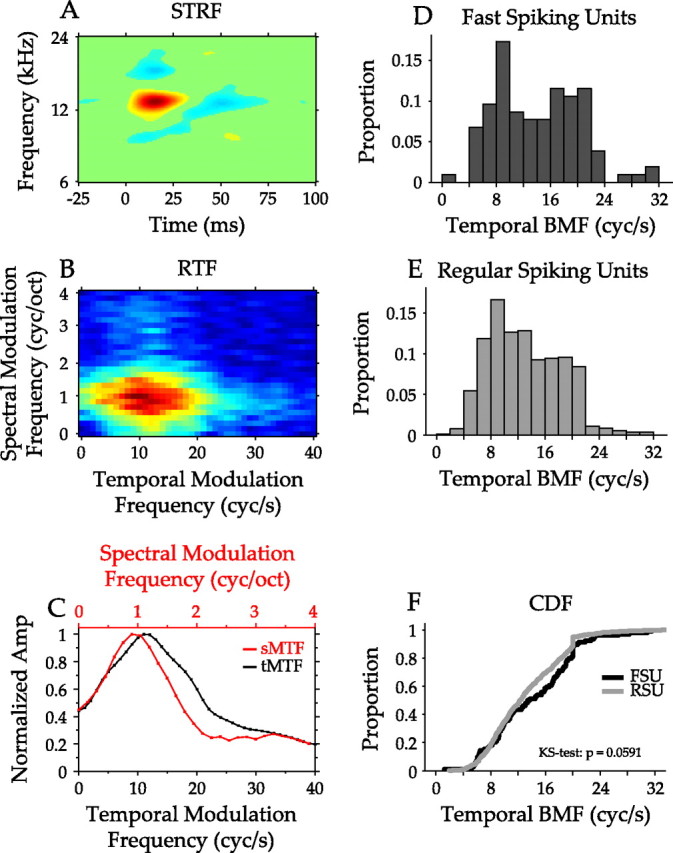
Analysis of modulation processing by FSUs and RSUs. A, STRF of a representative AI neuron. The abscissa represents time before a spike. The ordinate represents frequency. Suppression flanks the main excitatory component along the spectral and temporal axes. B, RTF of the STRF in A. The RTF describes the temporal and spectral modulation preferences of an AI neuron and is obtained through the 2D FFT of the STRF. The peak in the RTF is located at ∼10 cycles/s and 1 cycle/octave. C, Temporal and spectral modulation transfer functions obtained from the RTF. The temporal MTF (black) is obtained by summing the RTF across all spectral modulation frequencies. The spectral MTF (red) is obtained by summing across temporal modulation frequencies. The structure of the suppression in the STRF leads to the bandpass structure of the MTFs. D, Temporal best modulation frequency distribution for FSUs. The distribution is relatively uniform from 4 to 22 cycles/s. E, Temporal best modulation frequency distribution for RSUs. F, Comparison of the cumulative distribution functions for temporal best modulation frequency. The FSU and RSU distributions were not significantly different (p = 0.0591, KS test). The distributions for spectral best modulation frequency were also not significantly different (data not shown; p > 0.1, KS test).
Combining all recordings, the distributions of best temporal modulation frequency (bTMF) were similar for FSUs and RSUs (Fig. 6D,E). The distribution of bTMF values (FSU mean/SD, 14.1/6.15 Hz; RSU mean/SD, 13.0/5.25 Hz) spanned the range expected in AI, ∼4–24 Hz (Joris et al., 2004), and were not significantly different (Fig. 6F) (p = 0.059, KS test), although a trend toward lower RSU values was detected. Cumulative distributions of the encountered tMTF bandwidths were also not significantly different (data not shown; p = 0.208, KS test), nor were there differences in best spectral modulation frequency and spectral MTF width (data not shown; p = 0.230 and p = 0.109, respectively, KS test).
Best modulation frequency and MTF bandwidth are basic parameters characterizing temporal and spectral envelope filters (Joris et al., 2004). The overall shape of the MTF is another descriptor, which for auditory cortical neurons is usually in the form of low-pass or bandpass modulation filters. We found that FSU and RSU filter shapes were significantly different.
tMTFs were significantly more bandpass than low pass for FSUs, with 65% of FSUs having bandpass tMTFs compared with 47% of RSUs (Fig. 7, top). The difference was smaller but the result was the same for sMTFs, with 25% of FSUs and 15% of RSUs having bandpass sMTFs (Fig. 7, bottom). The null hypothesis was tested by pooling all FSU and RSU MTF shape data, for either temporal or spectral MTFs, and drawing 115 values from this distribution to represent simulated FSU data and 978 values for RSUs. From these groups, the bandpass percentages in the simulated FSU and RSU distributions were computed, and this process was repeated 25,000 times to form a resampled distribution. The observed percentages of bandpass MTFs were then compared with the resampled distribution, and it was found that FSU tMTFs were significantly more bandpass (p < 0.0001). In addition, more FSU sMTFs were bandpass (p = 0.016).
Figure 7.
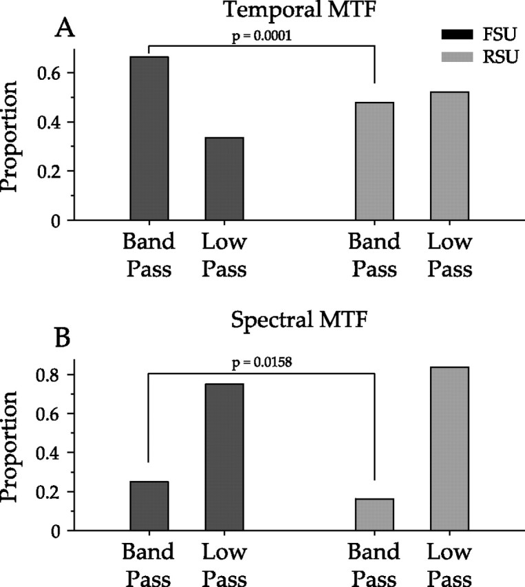
Analysis of modulation transfer function shapes for FSUs and RSUs. Temporal and spectral MTFs were classified as bandpass or low pass (see Materials and Methods). A resampling procedure was then used to determine whether the proportion of bandpass FSUs was significantly different from that of RSUs. Top, Temporal MTF shapes for FSUs and RSUs. A significantly greater proportion of FSUs (65%) compared with RSUs (47%) have bandpass tMTFs (p < 0.01). Bottom, A significantly larger proportion of FSU sMTFs (25%) were bandpass compared with RSUs (15%; p = 0.016).
STRF shape contains important information about the interaction between temporal and spectral processing aspects and may be quantified by the inseparability index. The index measures how well an STRF is approximated by a single pair of one-dimensional functions of frequency and time, respectively (Depireux et al., 2001). If the STRF must be approximated by multiple pairs of one-dimensional functions, the inseparability index will be ∼1, whereas values near 0 indicate that the approximation by a single pair of functions is appropriate, and thus, time and frequency may be dissociated in the STRF. Inseparability indices revealed significant differences in STRF shape for the two neuronal classes (FSU mean/SD, 0.36/0.18; RSU mean/SD, 0.44/0.18), with FSUs having more separable STRFs than RSUs (Fig. 8A,B).
Figure 8.

Analysis of FSU and RSU STRF structure. For each FSU or RSU, the structure of the STRF was quantified by determining the inseparability of each STRF. A, STRF inseparability analysis for two STRFs. The pair of independent one-dimensional functions that best approximates each STRF is shown. The procedure determines how time and frequency in the STRF may be dissociated. The left STRF is more inseparable (inseparability index of 0.22) than the right STRF (inseparability index of 0.15). B, Inseparability index cumulative distribution functions for FSU and RSU STRFs. Abscissa values near 0 represent STRFs that may be represented by one pair of one-dimensional functions, whereas values near 1 indicate that multiple pairs are required. The receptive fields of FSUs are significantly more separable than those of RSUs (p < 0.01, KS test).
Population comparisons using CDFs show the RSU distribution shifted to higher inseparability index values as well (Fig. 8B) (p < 0.01, KS test). Thus, the spiking property of a cell can predict some aspects of its spectrotemporal processing regime.
Although FSUs and RSUs differ in their spectrotemporal receptive field structure, these differences do not reveal the selectivity of each cell type for specific spectrotemporal stimulus patterns. We therefore computed FSIs, in which FSI values near 0 indicate a neuron unselective for spectrotemporal stimuli and values near 1 indicate a neuron responsive to few spectrotemporal patterns (Escabí et al., 2005). FSUs were significantly more feature selective (FSU mean/SD, 0.14/0.10; RSU mean/SD, 0.09/0.07) (Fig. 9A,B), as seen in the CDFs for both neuron types (p < 0.01, KS test) (Fig. 9C).
Figure 9.
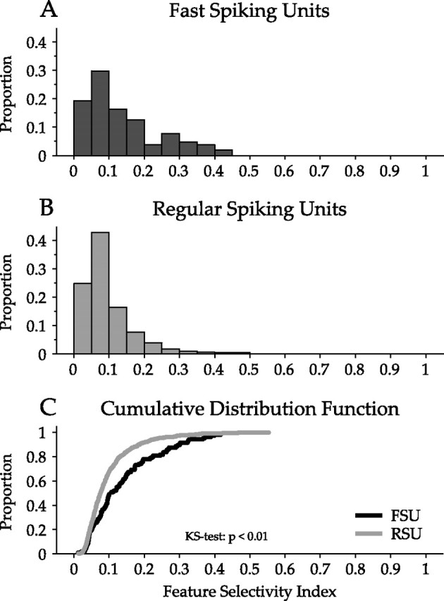
Analysis of feature selectivity of FSUs and RSUs. The FSI describes the stimulus specificity of a neuron. FSI values near 1 represent a neuron that is selective for only one stimulus feature, whereas values near 0 represent a neuron that is relatively unselective for specific spectrotemporal stimulus patterns. A, Distribution of feature selectivity indices for FSUs. The distribution extends to 0.45, representing moderately strong feature selectivity. B, The FSI distribution for RSUs. C, Comparison of FSI cumulative distribution functions. The FSU distribution is significantly shifted to higher FSIs values, indicating that FSUs are more selective for spectrotemporal stimulus features than RSUs (p < 0.01, KS test).
Nonlinearities
Only properties derived directly from the linearly accumulated STRFs have been examined. However, the relationship between stimulus, STRF, and neural response is often nonlinear. A nonlinear function applied to the linear filter can capture the relationship between the stimulus and the expected neural response. It describes the firing probability of a neuron as the similarity, or correlation, between the stimulus and the STRF changes (Fig. 10A) and forms a fundamental component in linear/nonlinear cascade models of neuronal function (Chichilnisky, 2001; Schwartz et al., 2006). From the example in Figure 10A, the firing rate increases as the similarity between segments of the dynamic moving ripple stimulus and the STRF increases. If the stimulus configuration and the filter (or STRF) properties are anticorrelated (negative abscissa values in Fig. 10A), the firing probability remains low, constituting an asymmetric nonlinearity. Asymmetric nonlinearities can be strongly monotonic (Fig. 10B), or the nonlinearity may plateau at higher similarity values (Fig. 10C). Nonmonotonic nonlinearities represent neurons selective for stimuli that are not optimally matched to the filter (Fig. 10D).
Figure 10.

Spectrotemporal processing model of auditory cortex neurons. A, The processing of AI neurons may be formulated in three steps: the dynamic moving ripple stimulus is processed by the STRF, the similarity, or correlation, between the STRF and the stimulus is determined, and the result is fed to a nonlinearity; and the nonlinearity determines the firing rate of the neuron as a function of the similarity between the stimulus and STRF. The units of the abscissa, in SDs, represent the likelihood of the stimulus–STRF similarity relative to that expected by a random stimulus. Thus, values near 5 represent stimuli that would be unlikely to be encountered by chance and expected from stimuli that lead to a spike response. B–D, Nonlinearities for three other neurons, displaying strongly monotonic, moderately monotonic, and nonmonotonic behavior. Dashed lines in nonlinearities represent the average firing rate of the neuron.
We quantitatively analyzed the skewness, monotonicity, and asymmetry of FSU and RSU nonlinearities. Skewness is the third central moment divided by the cube of the SD:
where Yi are the nonlinearity values, μ is the mean of the nonlinearity, N is the number of nonlinearity points, and σ is the SD of the nonlinearity. Skewness describes the amount of information in the tail of the nonlinearity. Gradual increases in firing rate with increasing stimulus–STRF correlation lead to a skewness near 1 (Fig. 11A), whereas skewness values are higher for nonlinearities with more rapidly increasing firing rates at higher similarity values (Fig. 11B). FSU skewness distributions were generally higher than for RSUs (Fig. 11C,D) (FSU mean/SD, 1.72/0.68; RSU mean/SD, 1.52/0.71). Analysis of the cumulative distribution showed the same result (Fig. 11E) (p < 0.01, KS test), which was validated by resampling analysis (Bain and Engelhardt, 1992). This finding suggests that the nonlinearities enable a higher feature selectivity of putative inhibitory interneurons compared with excitatory neurons.
Figure 11.

Skewness of nonlinearities. A, B, Two nonlinearities with different degrees of skewness. A, When the firing rate slowly increases with stimulus similarity the skewness is ∼1. B, When the rising portion of the nonlinearity is shifted to higher similarity values, the skewness increases to ∼3. C, D, Skewness distributions of FSU and RSU nonlinearities. FSU nonlinearities are shifted to more positive skewness values relative to RSUs. E, Cumulative distribution functions of FSU and RSU nonlinearity skewness values. The FSU distribution is significantly shifted to higher values (p < 0.01, KS test). F, Rank sum analysis of FSU/RSU skewness distributions. The rank sum statistic from the actual data were calculated (gray bar). Then, the FSU and RSU data were combined and resampled with respect to the number of FSUs and RSUs. From the resampled distributions the rank sum statistic was calculated. This process was repeated 10,000 times, and the histogram shows the distribution of these statistics, revealing significance (p = 0.0004).
The shape of the nonlinearities can be characterized by determining their monotonicity. If the spiking probability for at least the two highest stimulus-filter similarities was less than the maximum probability, the nonlinearity was classified as nonmonotonic. The majority of both FSU (69.6%) and RSU (64.4%) nonlinearities were monotonic (Fig. 12). The resampling analysis revealed no significant difference between the two cell groups (p > 0.01).
Figure 12.

Monotonicity of nonlinearities. Monotonicity was determined by first finding the maximum value in each nonlinearity, along with the following two nonlinearity values that corresponded to even higher stimulus similarity values. If the two values that followed the maximum were both less than the maximum value, then the nonlinearity was classified as nonmonotonic (Non-Mono). All other nonlinearities were classified as monotonic (Mono). A total of 69.6% of FSU and 64.4% of RSU nonlinearities were monotonic. Resampling the FSU and RSU distributions revealed that the difference in the proportion of monotonic nonlinearities between of FSUs and RSUs nonlinearities was not significant (p > 0.1).
Last, we examined the asymmetry of the nonlinearities. An asymmetry index (ASI) quantifies the difference in spiking probability for positive and negative correlations between stimulus and STRF. The ASI was defined as (R − L)/(R + L), where R and L are the sums of all nonlinearity values that correspond to similarity values greater than or less than 0, respectively. The index ranges from −1 to 1, with 0 representing a nonlinearity that is completely symmetric for positive and negative stimulus similarity values, implying that correlated and anticorrelated stimuli equally influence the probability of a neural response. ASIs near 1 or −1 indicate neurons that have an increased probability of spiking when the stimulus is either positively or negatively correlated with the filter, respectively. FSUs had nonlinearities that were more positively asymmetric than those of RSUs (Fig. 13) (FSU mean/SD, 0.84/0.17; RSU mean/SD, 0.76/0.17; p < 0.01, KS test; also confirmed by resampling). The higher asymmetry for FSUs again suggests that putative inhibitory interneurons tend toward higher feature selectivity, i.e., they prefer more complete matches between a spectrotemporal stimulus and filter features.
Figure 13.

Asymmetry of nonlinearities. The asymmetry index of each nonlinearity, which ranges from −1 to +1, was calculated by subtracting the sum of the nonlinearity values for negative STRF similarity values from those for positive values and dividing by the sum of the two. A, B, Distribution of FSU and RSU asymmetry index values. FSUs have a greater proportion of neurons with high asymmetry index values. C, Cumulative distribution functions of asymmetry index values. The FSU distribution is significantly shifted to higher values (p < 0.01, KS test). D, Rank sum analysis of asymmetry index values. The observed rank sum statistic (gray line) is significantly shifted from the resampled distribution (p < 0.01; n = 10,000), further indicating that FSU nonlinearities are more asymmetric than those for RSUs.
Interdependence of STRF characteristics
We have analyzed 10 main response characterizations based on STRFs and their associated nonlinearities to reveal differences between FSUs and RSUs. To assess whether these parameters covaried, we performed a factor analysis to determine which of the different parameters (firing rate, phase-locking index, best temporal modulation frequency, bandwidth of temporal MTF, spectral best modulation frequency, bandwidth of spectral MTF, inseparability index, features selectivity index, nonlinearity skewness, and nonlinearity asymmetry) could be treated independently. We pooled the FSU and RSU data separately and obtained the eigenvalues from the correlation matrix to estimate the number of independent factors that could best account for the variance in each dataset. Three independent factors emerged for both cell classes (eigenvalues >1.7) (Table 2). Additional factors had low eigenvalues (<0.9) and were not considered further. The three factors had the same basic composition for FSUs and RSUs. The largest factor revealed positive correlations between feature selectivity, phase-locking ability, and the asymmetry of the nonlinearity. Firing rate was negatively correlated with these parameters. This factor primarily captures response modes including response strength, timing, and stimulus specificity. The other two factors capture independently the spectral and temporal modulation preferences of the neurons, respectively. The distribution of individual neurons along these three factors was broad and unimodal, showing no unequivocal clustering that could be interpreted as functionally distinct neuronal subgroups. This finding suggests that FSU and RSU responses fall along a continuum, from low to high stimulus specificity, with accompanying changes in firing rate, timing precision, and nonlinearity asymmetry. This behavior is independent from any particular receptive field property, such as best temporal or spectral modulation frequency.
Table 2.
Factor analysis for FSUs and RSUs
| Factor 1 ″response mode″ FSU/RSU | Factor 2 ″spectral modulation″ FSU/RSU | Factor 3 ″temporal modulation″ FSU/RSU | |
|---|---|---|---|
| Eigenvalue | 3.72/3.44 | 2.41/2.14 | 1.74/1.92 |
| Firing rate | −0.63/−0.54 | −0.25/−0.18 | −0.10/−0.12 |
| Phase-locking index | 0.87/0.93 | −0.01/−0.07 | −0.40/−0.07 |
| Temporal BMF | 0.03/0.11 | −0.30/−0.06 | 0.80/0.84 |
| tMTF bandwidth | −0.03/−0.07 | −0.16/0.04 | 0.93/0.99 |
| Spectral BMF | 0.10/0.15 | 0.92/0.93 | −0.20/0.07 |
| sMTF bandwidth | 0.07/0.13 | 0.96/0.99 | −0.13/−0.05 |
| Inseparability index | −0.27/−0.29 | 0.35/0.40 | 0.46/0.28 |
| Feature selectivity index | 0.95/0.97 | 0.09/0.06 | −0.28/0.03 |
| Nonlinearity skewness | 0.45/0.43 | −0.03/0.00 | 0.06/-0.04 |
| Nonlinearity asymmetry index | 0.71/0.73 | −0.05/0.02 | −0.02/−0.02 |
The varimax orthogonal transformation was performed for 10 response and receptive field characterizations. Parameters with >20% variance contribution are shown in bold. FSU/RSU indicates the FSU value from one-factor analysis and the RSU value from another factor analysis.
Discussion
Inhibition has been implicated in multiple aspects of auditory cortical processing, including the establishment and shaping of frequency tuning. Although the frequency tuning of synaptic excitatory and inhibitory inputs is well matched (Wehr and Zador, 2003; Zhang et al., 2003), spike-based tuning curves are usually narrower than the frequency range of the synaptic inputs (Tan et al., 2004) and broaden with the application of a GABAA antagonist (Chang et al., 2005). This suggests that the shaping of spectral receptive fields may reflect specific interactions between excitatory and inhibitory synaptic components as well as biophysical mechanisms present in the spike-generating process (Wilent and Contreras, 2005).
Intensity tuning of cortical neurons, i.e., the nonmonotonic behavior of rate-level functions, can also be shaped or even created by an imbalance of cortical inhibition and excitation (Wu et al., 2006; Tan et al., 2007). In these cases, monotonic excitatory rate-level functions can be transformed into nonmonotonic membrane-potential growth, with inhibition dominating at higher sound levels (Tan et al., 2007).
The relative timing of excitatory and inhibitory inputs also plays a significant role in determining auditory cortical responses to more complex sounds. The direction selectivity for frequency modulation (FM) sweeps is correlated with the delay between excitatory and inhibitory inputs (Zhang et al., 2003). Furthermore, the relative timing between excitation and inhibition may affect spike precision (Wehr and Zador, 2003). Finally, the ability to change receptive field properties through plasticity mechanisms is enabled by inhibitory influences. Whole-cell recordings showed that short-term receptive field plasticity occurs when inhibition is reduced during the exposure to nonpreferred stimulus configurations (Froemke et al., 2007).
The current study showed that auditory cortical FSUs (putative inhibitory interneurons) differ from RSUs (putative excitatory pyramidal neurons) in nearly all investigated STRF properties and their associated nonlinearities (Table 1). Although many individual differences are relatively modest, combined they indicate a clear functional segregation between the two neuronal classes. Additionally, we found that cortical response behavior could be captured by three independent factors that equally apply to FSUs and RSUs (Table 2). The first factor encapsulates the response mode along a continuum of feature selectivity, firing rate, and spike-timing precision. The other two factors characterize the spectral and temporal modulation preferences of the neuron classes.
Classification of FSUs and RSUs
FSUs have been described in slice (McCormick et al., 1985; Rose and Metherate, 2005) and in both the anesthetized (Azouz et al., 1997; Andermann et al., 2004) and unanesthetized (de Ribaupierre et al., 1972; Simons, 1978; Volkov et al., 1989) in vivo preparations and, thus, represent categorical distinctions essentially independent from experimental procedures.
Spike-waveform-based identification of putative inhibitory interneurons, FSUs, is imperfect (Simons, 1978; Volkov et al., 1989; Andermann et al., 2004; Barthó et al., 2004) but shows excellent accord with anatomical results (McCormick et al., 1985; Kawaguchi and Kubota, 1993; Kawaguchi and Kondo, 2002; Swadlow, 2003). Intracellular recordings combined with morphological reconstructions and cytochemical analysis are required for a full identification but were not made in the present study, and thus some degree of classification error may be present. Our results apply only to FSUs and not other AI inhibitory neurons, because FSUs comprise a subset of neocortical GABAergic cells (Kawaguchi, 1993b; Kawaguchi and Kubota, 1993; Markram et al., 2004). Some pyramidal cells may also have short-duration action potentials that may create classification errors (Dykes et al., 1988; Gray and McCormick, 1996). Thus, although most FSUs are inhibitory neurons, the methodological concerns noted above have led to their classification as putative inhibitory interneurons (Swadlow, 1994, 1995).
Most cells had action potential waveforms consistent with RSUs, thus ∼90% of the cells in this study were likely pyramidal. In rabbit AI, ∼10% of layer 4 cells stain positively for parvalbumin (McMullen et al., 1994). We found that 13% (34 of 257) of the cells in layer 4 were FSUs, a class that includes parvalbumin-positive neurons (Kawaguchi and Kondo, 2002). This suggests a similar proportion of FSUs and RSUs in AI of cat and rabbit. Lower proportions of FSUs in layers 2/3 and upper layer 5 also echo distributions obtained in somatosensory and visual cortex (Demeulemeester et al., 1989; van Brederode et al., 1991).
Receptive field features
Excitatory sharpness of frequency tuning among simultaneously recorded FSUs and RSUs differed despite the similarity of local characteristic frequency. This is compatible with the notion that the spike-based tuning of RSUs, the potential synaptic target of FSUs, is narrower than their synaptic inputs (Tan et al., 2004).
Response latency was shorter for FSUs versus RSUs within a layer, perhaps enabling them to influence nearby cells with feedforward inhibition (Gabernet et al., 2005). This inhibition is likely to be strong, because FSUs receive stronger thalamocortical innervation than RSUs (Bruno and Simons, 2002). FSUs show greater phase locking to the spectrotemporal stimulus envelope and thus more precise spiking. Because FSUs may make somatic contact on pyramidal cells, the shorter latencies and high temporal precision of FSUs may control the temporal precision, response duration, and spectrotemporal response profile of other local neurons (Miles et al., 1996; Kawaguchi and Kubota, 1997; Zhang et al., 2003). The generation or shaping of intensity tuning (Tan et al., 2007) and FM direction selectivity (Zhang et al., 2003) may also reflect these FSU timing features.
Spectrotemporal receptive field features
Temporal and spectral modulations are prominent aspects of communication sounds. Tuning to particular modulation frequencies may help listeners to correctly identify speech (Drullman et al., 1994a,b; Drullman, 1995; Shannon et al., 1995; Smith et al., 2002). Likewise, spectral modulation information is important for communication sound processing because it is challenging for listeners to discriminate speech with degraded spectral envelopes (Leek et al., 1987; Shannon et al., 1998; Smith et al., 2002; Dreisbach et al., 2005). The global similarity of the FSU and RSU modulation properties indicates that they likely perform similar transformations of their thalamic modulation input, e.g., preferred spectral and temporal modulation frequency, and different transformations for others, such as the shape of MTFs. Connected thalamocortical neuron pairs often differ in their modulation properties (Miller et al., 2001b), and cortical modulation behavior may be shaped by local inhibitory mechanisms. However, the precise role of inhibition in determining temporal modulation behavior is still unclear (Kurt et al., 2006), and other factors, such as convergence of different modulation ranges and synaptic depression/facilitation, may play major roles in the generation of cortical modulation responses (Eggermont, 2002).
With regard to spectral modulation tuning, spectral MTF shape may remain constant as spectral contrast varies (Calhoun and Schreiner, 1998), and thus inhibition, with spectral modulation tuning matched to that of excitation, could contribute to cortical coding of vowel features, such as formants.
Separability and feature selectivity
STRF structure differs for FSUs and RSUs. FSU STRFs were more separable, thus more fully dissociating spectral and temporal processing because they can be approximated as the product of two independent functions. This implies less context dependence for spectral and temporal processing aspects than for RSUs. Whether this reflects different cortical connection patterns and/or different distributions and kinetic properties of GABAergic inputs to RSUs (Hefti and Smith, 2003) is unknown because detailed records of corticocortical inputs to inhibitory interneurons are not yet available.
FSUs had much higher feature selectivity indices than RSUs. Thus, FSUs respond to a much smaller stimulus set during the ripple stimulus, resulting in a lower overall firing rate for these neurons. Consequently, FSUs will likely have higher information values per spike than RSUs, because spike rate and information per spike are inversely related, as shown for a subset of inferior colliculus neurons (Escabí et al., 2005). These higher information values likely relate to FSU channel properties, because a likely contributor to greater feature selectivity is a higher spiking threshold for FSUs, similar to the high feature selectivity of inferior colliculus neurons (Escabí et al., 2005).
The lower feature selectivity of RSUs implies that they respond to a wider range of spectrotemporal patterns, suggesting increased context sensitivity (Fritz et al., 2003). FSUs transmit local information that is spectrotemporally restricted and temporally precise and, thus, are poised to play a crucial role in the dynamic properties of RSUs, including short-term and long-term spectrotemporal dynamics and plasticity (Fritz et al., 2003; Polley et al., 2006; Froemke et al., 2007).
Nonlinearities of FSUs and RSUs
The response probability of FSUs increases strongly as the correlation between the STRF and the stimulus grows, consistent with the finding that FSUs are more feature selective than RSUs. Feature selectivity in this context means that the variability of the stimuli eliciting a spike is decreased relative to that of RSUs. This decrease, combined with greater temporal precision and shorter latencies, places FSUs in a strong position to supply fast and temporally precise inhibition to neighboring cells (Gabernet et al., 2005).
Concluding remarks
A fundamental question of neocortex is how variations on a common excitatory template are used to accomplish the tasks native to each sensory system (Douglas and Martin, 2004). A component of this question may be addressed by examining the functional properties of inhibitory neurons in the microcircuit of different systems. In the visual cortex, inhibitory neurons have either simple or complex receptive fields (Azouz et al., 1997; Hirsch et al., 2003). There appears to be no significant difference between receptive field structure for putative inhibitory interneurons (FSUs) and putative excitatory neurons (RSUs) with respect to basket cells, a major FSU candidate (Hirsch et al., 2003). Parallels in receptive field structure of FSUs and RSUs in visual cortex contrast with auditory and somatosensory cortex, and specifically barrel cortex, in which basic receptive field properties diverge, and FSUs have larger bandwidths and different firing rates than RSUs (Simons, 1978; Simons and Carvell, 1989). The spectral integration of AI FSUs also seems broader than for RSUs, and the structure of the receptive fields and the temporal response precision differs between these neuron classes. Significantly, the biophysical properties of AI inhibitory neurons may be adapted for fast temporal processing, because the channel kinetics of AI neurons are faster than those in other sensory systems (Hefti and Smith, 2003). Thus, in total, the current study provides a preliminary description of the differences in spectrotemporal processing between FSUs and RSUs and begins to resolve the functional role of inhibition in auditory cortex.
Footnotes
This work was supported by National Institutes of Health Grants DC02260 and MH 077970 and by Hearing Research (San Francisco, CA). We thank Andrew Tan, Marc Heiser, Kazuo Imaizumi, and Benedicte Philibert for experimental assistance; Mark Kvale for the use of his SpikeSort1.3 Bayesian spike-sorting software; and Jeff Winer for previous comments on this manuscript.
References
- Aertsen A, Johannesma PI. Spectro-temporal receptive fields of auditory neurons in the grassfrog. I. Characterization of tonal and natural stimuli. Biol Cybern. 1980;38:223–234. doi: 10.1007/BF00342772. [DOI] [PubMed] [Google Scholar]
- Aguera y Arcas B, Fairhall AL, Bialek W. Computation in a single neuron: Hodgkin and Huxley revisited. Neural Comput. 2003;15:1715–1749. doi: 10.1162/08997660360675017. [DOI] [PubMed] [Google Scholar]
- Andermann ML, Ritt J, Neimark MA, Moore CI. Neural correlates of vibrissa resonance; band-pass and somatotopic representation of high-frequency stimuli. Neuron. 2004;42:451–463. doi: 10.1016/s0896-6273(04)00198-9. [DOI] [PubMed] [Google Scholar]
- Attwell D, Laughlin SB. An energy budget for signaling in the grey matter of the brain. J Cereb Blood Flow Metab. 2001;21:1133–1145. doi: 10.1097/00004647-200110000-00001. [DOI] [PubMed] [Google Scholar]
- Azouz R, Gray CM, Nowak LG, McCormick DA. Physiological properties of inhibitory interneurons in cat striate cortex. Cereb Cortex. 1997;7:534–545. doi: 10.1093/cercor/7.6.534. [DOI] [PubMed] [Google Scholar]
- Baddeley R, Abbott LF, Booth MC, Sengpiel F, Freeman T, Wakeman EA, Rolls ET. Responses of neurons in primary and inferior temporal visual cortices to natural scenes. Proc Biol Sci. 1997;264:1775–1783. doi: 10.1098/rspb.1997.0246. [DOI] [PMC free article] [PubMed] [Google Scholar]
- Bain LJ, Engelhardt M. Ed 2. Boston: PWS-KENT; 1992. Introduction to probability and mathematical statistics. [Google Scholar]
- Barthó P, Hirase H, Monconduit L, Zugaro M, Harris KD, Buzsáki G. Characterization of neocortical principal cells and interneurons by network interactions and extracellular features. J Neurophysiol. 2004;92:600–608. doi: 10.1152/jn.01170.2003. [DOI] [PubMed] [Google Scholar]
- Bruno RM, Simons DJ. Feedforward mechanisms of excitatory and inhibitory cortical receptive fields. J Neurosci. 2002;22:10966–10975. doi: 10.1523/JNEUROSCI.22-24-10966.2002. [DOI] [PMC free article] [PubMed] [Google Scholar]
- Calhoun BM, Schreiner CE. Spectral envelope coding in cat primary auditory cortex: linear and non-linear effects of stimulus characteristics. Eur J Neurosci. 1998;10:926–940. doi: 10.1046/j.1460-9568.1998.00102.x. [DOI] [PubMed] [Google Scholar]
- Callaway EM. Local circuits in primary visual cortex of the macaque monkey. Annu Rev Neurosci. 1998;21:47–74. doi: 10.1146/annurev.neuro.21.1.47. [DOI] [PubMed] [Google Scholar]
- Callaway EM. Feedforward, feedback and inhibitory connections in primate visual cortex. Neural Netw. 2004;17:625–632. doi: 10.1016/j.neunet.2004.04.004. [DOI] [PubMed] [Google Scholar]
- Chang EF, Bao S, Imaizumi K, Schreiner CE, Merzenich MM. Development of spectral and temporal response selectivity in the auditory cortex. Proc Natl Acad Sci USA. 2005;102:16460–16465. doi: 10.1073/pnas.0508239102. [DOI] [PMC free article] [PubMed] [Google Scholar]
- Chichilnisky EJ. A simple white noise analysis of neuronal light responses. Network. 2001;12:199–213. [PubMed] [Google Scholar]
- Cruikshank SJ, Lewis TJ, Connors BW. Synaptic basis for intense thalamocortical activation of feedforward inhibitory cells in neocortex. Nat Neurosci. 2007;10:462–468. doi: 10.1038/nn1861. [DOI] [PubMed] [Google Scholar]
- deCharms RC, Blake DT, Merzenich MM. Optimizing sound features for cortical neurons. Science. 1998;280:1439–1443. doi: 10.1126/science.280.5368.1439. [DOI] [PubMed] [Google Scholar]
- Demeulemeester H, Vandesande F, Orban GA, Heizmann CW, Pochet R. Calbindin D-28K and parvalbumin immunoreactivity is confined to two separate neuronal subpopulations in the cat visual cortex, whereas partial coexistence is shown in the dorsal lateral geniculate nucleus. Neurosci Lett. 1989;99:6–11. doi: 10.1016/0304-3940(89)90255-3. [DOI] [PubMed] [Google Scholar]
- Depireux DA, Simon JZ, Klein DJ, Shamma SA. Spectro-temporal response field characterization with dynamic ripples in ferret primary auditory cortex. J Neurophysiol. 2001;85:1220–1234. doi: 10.1152/jn.2001.85.3.1220. [DOI] [PubMed] [Google Scholar]
- de Ribaupierre F, Goldstein MH, Jr, Yeni-Komshian G. Cortical coding of repetitive acoustic pulses. Brain Res. 1972;48:205–225. doi: 10.1016/0006-8993(72)90179-5. [DOI] [PubMed] [Google Scholar]
- Douglas RJ, Martin KAC. Neuronal circuits of the neocortex. Annu Rev Neurosci. 2004;27:419–451. doi: 10.1146/annurev.neuro.27.070203.144152. [DOI] [PubMed] [Google Scholar]
- Dreisbach LE, Leek MR, Lentz JJ. Perception of spectral contrast by hearing-impaired listeners. J Speech Lang Hear Res. 2005;48:910–921. doi: 10.1044/1092-4388(2005/063). [DOI] [PubMed] [Google Scholar]
- Drullman R. Temporal envelope and fine structure cues for speech intelligibility. J Acoust Soc Am. 1995;97:585–592. doi: 10.1121/1.413112. [DOI] [PubMed] [Google Scholar]
- Drullman R, Festen JM, Plomp R. Effect of temporal envelope smearing on speech reception. J Acoust Soc Am. 1994a;95:1053–1064. doi: 10.1121/1.408467. [DOI] [PubMed] [Google Scholar]
- Drullman R, Festen JM, Plomp R. Effect of reducing slow temporal modulations on speech reception. J Acoust Soc Am. 1994b;95:2670–2680. doi: 10.1121/1.409836. [DOI] [PubMed] [Google Scholar]
- Dykes RW, Lamour Y, Diadori P, Landry P, Dutar P. Somatosensory cortical neurons with an identifiable electrophysiological signature. Brain Res. 1988;441:45–58. doi: 10.1016/0006-8993(88)91382-0. [DOI] [PubMed] [Google Scholar]
- Eggermont JJ. Temporal modulation transfer functions in cat primary auditory cortex: separating stimulus effects from neural mechanisms. J Neurophysiol. 2002;87:305–321. doi: 10.1152/jn.00490.2001. [DOI] [PubMed] [Google Scholar]
- Escabí MA, Schreiner CE. Nonlinear spectrotemporal sound analysis by neurons in the auditory midbrain. J Neurosci. 2002;22:4114–4131. doi: 10.1523/JNEUROSCI.22-10-04114.2002. [DOI] [PMC free article] [PubMed] [Google Scholar]
- Escabí MA, Nassiri R, Miller LM, Schreiner CE, Read HL. The contribution of spike threshold to acoustic feature selectivity, spike information content, and information throughput. J Neurosci. 2005;25:9524–9534. doi: 10.1523/JNEUROSCI.1804-05.2005. [DOI] [PMC free article] [PubMed] [Google Scholar]
- Fairén A, DeFelipe J, Regidor J. Nonpyramidal neurons. In: Peters A, Jones EG, editors. Cerebral cortex. New York: Plenum; 1984. pp. 201–253. [Google Scholar]
- Fritz J, Shamma S, Elhilali M, Klein D. Rapid task-related plasticity of spectrotemporal receptive fields in primary auditory cortex. Nat Neurosci. 2003;6:1216–1223. doi: 10.1038/nn1141. [DOI] [PubMed] [Google Scholar]
- Froemke RC, Merzenich MM, Schreiner CE. A synaptic memory trace for cortical receptive field plasticity. Nature. 2007;450:425–429. doi: 10.1038/nature06289. [DOI] [PubMed] [Google Scholar]
- Gabernet L, Jadhav SP, Feldman DE, Carandini M, Scanziani M. Somatosensory integration controlled by dynamic thalamocortical feed-forward inhibition. Neuron. 2005;48:315–327. doi: 10.1016/j.neuron.2005.09.022. [DOI] [PubMed] [Google Scholar]
- Gray CM, McCormick DA. Chattering cells: superficial pyramidal neurons contributing to the generation of synchronous oscillations in the visual cortex. Science. 1996;274:109–113. doi: 10.1126/science.274.5284.109. [DOI] [PubMed] [Google Scholar]
- Hefti BJ, Smith PH. Distribution and kinetic properties of GABAergic inputs to layer V pyramidal cells in rat auditory cortex. J Assoc Res Otolaryngol. 2003;4:106–121. doi: 10.1007/s10162-002-3012-z. [DOI] [PMC free article] [PubMed] [Google Scholar]
- Hendry SH, Jones EG. GABA neuronal subpopulations in cat primary auditory cortex: co-localization with calcium binding proteins. Brain Res. 1991;543:45–55. doi: 10.1016/0006-8993(91)91046-4. [DOI] [PubMed] [Google Scholar]
- Hirsch JA, Martinez LM, Pillai C, Alonso JM, Wang Q, Sommer FT. Functionally distinct inhibitory neurons at the first stage of visual cortical processing. Nat Neurosci. 2003;6:1300–1308. doi: 10.1038/nn1152. [DOI] [PubMed] [Google Scholar]
- Holmgren C, Harkany T, Svennenfors B, Zilberter Y. Pyramidal cell communication within local networks in layer 2/3 of rat neocortex. J Physiol (Lond) 2003;551:139–153. doi: 10.1113/jphysiol.2003.044784. [DOI] [PMC free article] [PubMed] [Google Scholar]
- Houser CR, Vaughan JE, Hendry SH, Jones EG, Peters A. GABA neurons in the cerebral cortex. In: Jones EG, Peters A, editors. Cerebral cortex. New York: Plenum; 1984. pp. 63–89. [Google Scholar]
- Joris PX, Schreiner CE, Rees A. Neural processing of amplitude-modulated sounds. Physiol Rev. 2004;84:541–577. doi: 10.1152/physrev.00029.2003. [DOI] [PubMed] [Google Scholar]
- Kawaguchi Y. Physiological, morphological, and histochemical characterization of three classes of interneurons in rat neostriatum. J Neurosci. 1993a;13:4908–4923. doi: 10.1523/JNEUROSCI.13-11-04908.1993. [DOI] [PMC free article] [PubMed] [Google Scholar]
- Kawaguchi Y. Groupings of nonpyramidal and pyramidal cells with specific physiological and morphological characteristics in rat frontal cortex. J Neurophysiol. 1993b;69:416–431. doi: 10.1152/jn.1993.69.2.416. [DOI] [PubMed] [Google Scholar]
- Kawaguchi Y, Kondo S. Parvalbumin, somatostatin and cholecystokinin as chemical markers for specific GABAergic interneuron types in the rat frontal cortex. J Neurocytol. 2002;31:277–287. doi: 10.1023/a:1024126110356. [DOI] [PubMed] [Google Scholar]
- Kawaguchi Y, Kubota Y. Correlation of physiological subgroupings of nonpyramidal cells with parvalbumin- and calbindinD28k-immunoreactive neurons in layer V of rat frontal cortex. J Neurophysiol. 1993;70:387–396. doi: 10.1152/jn.1993.70.1.387. [DOI] [PubMed] [Google Scholar]
- Kawaguchi Y, Kubota Y. GABAergic cell subtypes and their synaptic connections in rat frontal cortex. Cereb Cortex. 1997;7:476–486. doi: 10.1093/cercor/7.6.476. [DOI] [PubMed] [Google Scholar]
- Klein DJ, Depireux DA, Simon JZ, Shamma SA. Robust spectrotemporal reverse correlation for the auditory system: optimizing stimulus design. J Comput Neurosci. 2000;9:85–111. doi: 10.1023/a:1008990412183. [DOI] [PubMed] [Google Scholar]
- Kurt S, Crook JM, Ohl FW, Scheich H, Schulze H. Differential effects of iontophoretic in vivo application of the GABA(A)-antagonists bicuculline and gabazine in sensory cortex. Hear Res. 2006;212:224–235. doi: 10.1016/j.heares.2005.12.002. [DOI] [PubMed] [Google Scholar]
- Leek MR, Dorman MF, Summerfield Q. Minimum spectral contrast for vowel identification by normal-hearing and hearing-impaired listeners. J Acoust Soc Am. 1987;81:148–154. doi: 10.1121/1.395024. [DOI] [PubMed] [Google Scholar]
- Lennie P. The cost of cortical computation. Curr Biol. 2003;13:493–497. doi: 10.1016/s0960-9822(03)00135-0. [DOI] [PubMed] [Google Scholar]
- Lewicki MS. Bayesian modeling and classification of neural signals. Neural Comput. 1994;6:1005–1030. [Google Scholar]
- Markram H, Toledo-Rodriguez M, Wang Y, Gupta A, Silberberg G, Wu C. Interneurons of the neocortical inhibitory system. Nat Rev Neurosci. 2004;5:793–807. doi: 10.1038/nrn1519. [DOI] [PubMed] [Google Scholar]
- McCormick DA, Connors BW, Lighthall JW, Prince DA. Comparative electrophysiology of pyramidal and sparsely spiny stellate neurons of the neocortex. J Neurophysiol. 1985;54:782–806. doi: 10.1152/jn.1985.54.4.782. [DOI] [PubMed] [Google Scholar]
- McMullen NT, Smelser CB, de Venecia RK. A quantitative analysis of parvalbumin neurons in rabbit auditory neocortex. J Comp Neurol. 1994;349:493–511. doi: 10.1002/cne.903490402. [DOI] [PubMed] [Google Scholar]
- Miles R, Toth K, Gulyas AI, Hajos N, Freund TF. Differences between somatic and dendritic inhibition in the hippocampus. Neuron. 1996;16:815–823. doi: 10.1016/s0896-6273(00)80101-4. [DOI] [PubMed] [Google Scholar]
- Miller KD. Understanding layer 4 of the cortical circuit: a model based on cat V1. Cereb Cortex. 2003;13:73–82. doi: 10.1093/cercor/13.1.73. [DOI] [PubMed] [Google Scholar]
- Miller LM, Schreiner CE. Stimulus-based state control in the thalamocortical system. J Neurosci. 2000;20:7011–7016. doi: 10.1523/JNEUROSCI.20-18-07011.2000. [DOI] [PMC free article] [PubMed] [Google Scholar]
- Miller LM, Escabí MA, Schreiner CE. Feature selectivity and interneuronal cooperation in the thalamocortical system. J Neurosci. 2001a;21:8136–8144. doi: 10.1523/JNEUROSCI.21-20-08136.2001. [DOI] [PMC free article] [PubMed] [Google Scholar]
- Miller LM, Escabí MA, Read HL, Schreiner CE. Functional convergence of response properties in the auditory thalamocortical system. Neuron. 2001b;32:151–160. doi: 10.1016/s0896-6273(01)00445-7. [DOI] [PubMed] [Google Scholar]
- Miller LM, Escabí MA, Read HL, Schreiner CE. Spectrotemporal receptive fields in the lemniscal auditory thalamus and cortex. J Neurophysiol. 2002;87:516–527. doi: 10.1152/jn.00395.2001. [DOI] [PubMed] [Google Scholar]
- Mitani A, Shimokouchi M. Neuronal connections in the primary auditory cortex: an electrophysiological study in the cat. J Comp Neurol. 1985;235:417–429. doi: 10.1002/cne.902350402. [DOI] [PubMed] [Google Scholar]
- Mitani A, Shimokouchi M, Itoh K, Nomura S, Kudo M, Mizuno N. Morphology and laminar organization of electrophysiologically identified neurons in the primary auditory cortex in the cat. J Comp Neurol. 1985;235:430–447. doi: 10.1002/cne.902350403. [DOI] [PubMed] [Google Scholar]
- Mitchell JF, Sundberg KA, Reynolds JH. Differential attention-dependent response modulation across cell classes in macaque visual area V4. Neuron. 2007;55:131–141. doi: 10.1016/j.neuron.2007.06.018. [DOI] [PubMed] [Google Scholar]
- Polley DB, Steinberg EE, Merzenich MM. Perceptual learning directs auditory cortical map reorganization through top-down influences. J Neurosci. 2006;26:4970–4982. doi: 10.1523/JNEUROSCI.3771-05.2006. [DOI] [PMC free article] [PubMed] [Google Scholar]
- Rose HJ, Metherate R. Auditory thalamocortical transmission is reliable and temporally precise. J Neurophysiol. 2005;94:2019–2030. doi: 10.1152/jn.00860.2004. [DOI] [PubMed] [Google Scholar]
- Schreiner CE, Mendelson JR. Functional topography of cat primary auditory cortex: distribution of integrated excitation. J Neurophysiol. 1990;64:1442–1459. doi: 10.1152/jn.1990.64.5.1442. [DOI] [PubMed] [Google Scholar]
- Schwartz O, Pillow JW, Rust NC, Simoncelli EP. Spike-triggered neural characterization. J Vis. 2006;6:484–507. doi: 10.1167/6.4.13. [DOI] [PubMed] [Google Scholar]
- Shannon RV, Zeng FG, Kamath V, Wygonski J, Ekelid M. Speech recognition with primarily temporal cues. Science. 1995;270:303–304. doi: 10.1126/science.270.5234.303. [DOI] [PubMed] [Google Scholar]
- Shannon RV, Zeng FG, Wygonski J. Speech recognition with altered spectral distribution of envelope cues. J Acoust Soc Am. 1998;104:2467–2476. doi: 10.1121/1.423774. [DOI] [PubMed] [Google Scholar]
- Silberberg G, Markram H. Disynaptic inhibition between neocortical pyramidal cells mediated by Martinotti cells. Neuron. 2007;53:735–746. doi: 10.1016/j.neuron.2007.02.012. [DOI] [PubMed] [Google Scholar]
- Simons DJ. Response properties of vibrissa units in rat SI somatosensory neocortex. J Neurophysiol. 1978;41:798–820. doi: 10.1152/jn.1978.41.3.798. [DOI] [PubMed] [Google Scholar]
- Simons DJ, Carvell GE. Thalamocortical response transformation in the rat vibrissa/barrel system. J Neurophysiol. 1989;61:311–330. doi: 10.1152/jn.1989.61.2.311. [DOI] [PubMed] [Google Scholar]
- Smith ZM, Delgutte B, Oxenham AJ. Chimaeric sounds reveal dichotomies in auditory perception. Nature. 2002;416:87–90. doi: 10.1038/416087a. [DOI] [PMC free article] [PubMed] [Google Scholar]
- Sugino K, Hempel CM, Miller MN, Hattox AM, Shapiro P, Wu C, Huang ZJ, Nelson SB. Molecular taxonomy of major neuronal classes in the adult mouse forebrain. Nat Neurosci. 2006;9:99–107. doi: 10.1038/nn1618. [DOI] [PubMed] [Google Scholar]
- Swadlow HA. Efferent neurons and suspected interneurons in motor cortex of the awake rabbit: axonal properties, sensory receptive fields, and subthreshold synaptic inputs. J Neurophysiol. 1994;71:437–453. doi: 10.1152/jn.1994.71.2.437. [DOI] [PubMed] [Google Scholar]
- Swadlow HA. Influence of VPM afferents on putative inhibitory interneurons in S1 of the awake rabbit: evidence from cross-correlation, microstimulation, and latencies to peripheral sensory stimulation. J Neurophysiol. 1995;73:1584–1599. doi: 10.1152/jn.1995.73.4.1584. [DOI] [PubMed] [Google Scholar]
- Swadlow HA. Fast-spike interneurons and feedforward inhibition in awake sensory neocortex. Cereb Cortex. 2003;13:25–32. doi: 10.1093/cercor/13.1.25. [DOI] [PubMed] [Google Scholar]
- Tan AY, Zhang LI, Merzenich MM, Schreiner CE. Tone-evoked excitatory and inhibitory synaptic conductances of primary auditory cortex neurons. J Neurophysiol. 2004;92:630–643. doi: 10.1152/jn.01020.2003. [DOI] [PubMed] [Google Scholar]
- Tan AY, Atencio CA, Polley DB, Merzenich MM, Schreiner CE. Unbalanced synaptic inhibition can create intensity-tuned auditory cortex neurons. Neuroscience. 2007;146:449–462. doi: 10.1016/j.neuroscience.2007.01.019. [DOI] [PubMed] [Google Scholar]
- Theunissen FE, Sen K, Doupe AJ. Spectral-temporal receptive fields of nonlinear auditory neurons obtained using natural sounds. J Neurosci. 2000;20:2315–2331. doi: 10.1523/JNEUROSCI.20-06-02315.2000. [DOI] [PMC free article] [PubMed] [Google Scholar]
- Thomson AM, West DC, Wang Y, Bannister AP. Synaptic connections and small circuits involving excitatory and inhibitory neurons in layers 2–5 of adult rat and cat neocortex: triple intracellular recordings and biocytin labelling in vitro. Cereb Cortex. 2002;12:936–953. doi: 10.1093/cercor/12.9.936. [DOI] [PubMed] [Google Scholar]
- Toledo-Rodriguez M, Blumenfeld B, Wu C, Luo J, Attali B, Goodman P, Markram H. Correlation maps allow neuronal electrical properties to be predicted from single-cell gene expression profiles in rat neocortex. Cereb Cortex. 2004;14:1310–1327. doi: 10.1093/cercor/bhh092. [DOI] [PubMed] [Google Scholar]
- van Brederode JF, Helliesen MK, Hendrickson AE. Distribution of the calcium-binding proteins parvalbumin and calbindin-D28k in the sensorimotor cortex of the rat. Neuroscience. 1991;44:157–171. doi: 10.1016/0306-4522(91)90258-p. [DOI] [PubMed] [Google Scholar]
- Volkov IO, Galazyuk AV, Dembnovetskii OF. Interaction of neurons characterized by a tonic reaction to sound with other neurons in the cat auditory cortex (in Russian) Neirofiziologiia. 1989;21:613–620. [PubMed] [Google Scholar]
- Wang Y, Gupta A, Toledo-Rodriguez M, Wu CZ, Markram H. Anatomical, physiological, molecular and circuit properties of nest basket cells in the developing somatosensory cortex. Cereb Cortex. 2002;12:395–410. doi: 10.1093/cercor/12.4.395. [DOI] [PubMed] [Google Scholar]
- Wang Y, Toledo-Rodriguez M, Gupta A, Wu C, Silberberg G, Luo J, Markram H. Anatomical, physiological and molecular properties of Martinotti cells in the somatosensory cortex of the juvenile rat. J Physiol (Lond) 2004;561:65–90. doi: 10.1113/jphysiol.2004.073353. [DOI] [PMC free article] [PubMed] [Google Scholar]
- Wehr M, Zador AM. Balanced inhibition underlies tuning and sharpens spike timing in auditory cortex. Nature. 2003;426:442–446. doi: 10.1038/nature02116. [DOI] [PubMed] [Google Scholar]
- Wilent WB, Contreras D. Stimulus-dependent changes in spike threshold enhance feature selectivity in rat barrel cortex neurons. J Neurosci. 2005;25:2983–2991. doi: 10.1523/JNEUROSCI.4906-04.2005. [DOI] [PMC free article] [PubMed] [Google Scholar]
- Winer JA. The functional architecture of the medial geniculate body and the primary auditory cortex. In: Webster DB, Popper AN, Fay RR, editors. The mammalian auditory pathway: neuroanatomy. New York: Springer; 1992. pp. 222–409. [Google Scholar]
- Wise KD. Silicon microsystems for neuroscience and neural prostheses. IEEE Eng Med Biol Soc. 2005;24:22–29. doi: 10.1109/memb.2005.1511497. [DOI] [PubMed] [Google Scholar]
- Wu GK, Li P, Tao HW, Zhang LI. Nonmonotonic synaptic excitation and imbalanced inhibition underlying cortical intensity tuning. Neuron. 2006;52:705–715. doi: 10.1016/j.neuron.2006.10.009. [DOI] [PMC free article] [PubMed] [Google Scholar]
- Zhang LI, Tan AY, Schreiner CE, Merzenich MM. Topography and synaptic shaping of direction selectivity in primary auditory cortex. Nature. 2003;424:201–205. doi: 10.1038/nature01796. [DOI] [PubMed] [Google Scholar]