

SUMMARY
Single-cell RNA-sequencing has become a widely used, powerful approach for studying cell populations. However, these methods often generate multiplet artifacts, where two or more cells receive the same barcode, resulting in a hybrid transcriptome. In most experiments, multiplets account for several percent of transcriptomes and can confound downstream data analysis. Here, we present Single-Cell Remover of Doublets (Scrublet), a framework for predicting the impact of multiplets in a given analysis and identifying problematic multiplets. Scrublet avoids the need for expert knowledge or cell clustering by simulating multiplets from the data and building a nearest neighbor classifier. To demonstrate the utility of this approach, we test Scrublet on several datasets that include independent knowledge of cell multiplets. Scrublet is freely available for download at github.com/AllonKleinLab/scrublet.
Graphical Abstract
In Brief
Single-cell RNA-sequencing experiments generate “multiplet errors” when multiple cells are labeled with the same barcode. Wolock et al. describe Scrublet, a method for predicting the effects of multiplets on downstream analyses and identifying problematic multiplets. They validate the method by applying Scrublet to several datasets with independent knowledge of multiplets.
INTRODUCTION
Single-cell RNA-sequencing (scRNA-seq) is a powerful and accessible approach for studying complex biological systems. It is quickly becoming a standard tool for unbiased characterization of tissue cell types and high-resolution reconstruction of differentiation trajectories (Griffiths et al., 2018). Droplet microfluidic (Klein et al., 2015; Macosko et al., 2015; Zheng et al., 2017) and well-based (Cao et al., 2017; Gierahn et al., 2017; Han et al., 2018; Rosenberg et al., 2018) technologies now enable the relatively inexpensive, high-throughput isolation and barcoding of cell transcriptomes. However, these methods suffer from the problem of cell multiplets, where a mixture of two or more cells is reported as a single cell in the data.
Most scRNA-seq technologies co-encapsulate cells and barcoded primers in a small reaction volume (droplets or wells), thereby associating the mRNA of each cell with a unique DNA barcode. Multiplets arise when two or more cells are captured within the same reaction, generating a hybrid transcriptome (Figure 1A). Cell multiplets are a concern when interpreting the outcome of scRNA-seq experiments because they suggest the existence of intermediate cell states that may not actually exist in the sample. Such artifactual states can confound downstream analyses by appearing as distinct cell types, bridging cell states, or interfering in differential gene expression tests and inference of gene regulatory networks (Figure 1B).
Figure 1. A Computational Approach for Identifying Doublets in Single-Cell RNA-Seq Data.
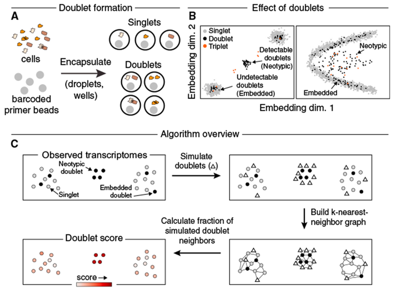
(A) Schematic of doublet formation. Multiple cells are co-encapsulated with a single barcoded bead, either randomly or as aggregates, resulting in the generation of a hybrid transcriptome.
(B) Multiplets involving highly similar cells (“embedded”) may be difficult to distinguish from single cells, while multiplets of dissimilar cells (“neotypic”) generate qualitatively new features, such as distinct clusters (left) or bridges (right).
(C) Overview of the Scrublet algorithm. Doublets are simulated by randomly sampling and combining observed transcriptomes, and the local density of simulated doublets, as measured by a nearest neighbor graph, is used to calculate a doublet score for each observed transcriptome.
In a typical scRNA-seq experiment, at least several percent of all capture events are multiplets (Cao et al., 2017; Klein et al., 2015; Macosko et al., 2015; Zheng et al., 2017). Multiplets can form as a result of cell aggregates or through random co-encapsulation of more than one cell per droplet or well. The rate of random co-encapsulation can be reduced by processing very dilute cell suspensions. However, in practice, it is often favorable to work with high cell concentrations in order to capture a large number of cells within a short amount of time and to reduce reagent costs. Additionally, multiplets resulting from cell aggregates cannot be eliminated by simply reducing cell concentration. Pre-sorting cells into wells can overcome these problems (Jaitin et al., 2014; Picelli et al., 2013) but at a cost in throughput. Thus, rather than avoiding multiplets, it would be useful to identify them, either computationally or through experimental means.
The Case for a Computational Approach to Multiplet Inference
Ideally, one would identify multiplet events experimentally through appropriate assay designs. At the time of writing, we noted five existing experimental strategies for multiplet detection, summarized in Table 1. However, none of the existing methods can yet be implemented routinely for all scRNA-seq experimental designs (see “Limitations” in Table 1). It would therefore be useful to have a computational strategy to infer the identity of multiplets directly from data.
Table 1.
Experimental Methods for Multiplet Detection
| Method name and references | Approach | Limitations |
|---|---|---|
|
Species mixing (Klein et al., 2015; Macosko et al., 2015) |
Cells from different species (e.g., mouse and human) are mixed and barcoded. Multiplets are detected as cell barcodes associated with transcripts from both species. Assuming 1:1 mixing, the identified multiplets represent half of all multiplets, as the remaining half are intra-species multiplets. | • Measures multiplet rate but does not facilitate detection of multiplet cell states in typical experimental samples from a single organism |
|
Natural genetic
variation (Kang et al., 2018; Xu etal., 2019) |
By mixing together cells from comparable samples from multiple genotyped individuals, genetic variants in transcripts can be used to assign each cell barcode to one individual, or in the case of multiplets, to multiple individuals. Only inter-individual multiplets can be identified, so the fraction of detectable multiplets increases with the number of individuals. | • Limited to samples with high genetic
diversity • Only possible if samples from different individuals can be pooled and assayed simultaneously |
|
Genetic
labeling (Adamson et al., 2016; Datlinger et al., 2017; Guo et al., 2019) |
Unique, expressed, genetic labels are introduced into the cell sample prior to collection. Multiplets can then be detected as cell barcodes with multiple distinct genetic labels. | • Introduction of genetic labels is
currently possible only for cultured cells or limited in
vivo conditions • Labeling may perturb the cells |
| Cell “hashing” (Gehring et al., 2018; Stoeckius et al., 2018; McGinnis et al., 2018) |
Cells are split into multiple wells, and each is labeled with sample-specific oligonucleotide tags, using antibodies or chemical approaches. Samples are then pooled prior to scRNA-seq. Multiplets are identified as cell barcodes associated with multiple oligo sequences. | • Not well suited for very small or fragile samples that cannot be split and recombined |
| Cell encapsulation at multiple cell concentrations | After processing the same input sample at multiple cell concentrations, multiplet-specific cell states can be detected by finding cell states whose proportion increases with the cell concentration. | • Requires at least two runs for each
sample • Requires sufficient cells |
Until now, two simple computational methods have been implemented to exclude putative multiplets: (1) exclude cell barcodes with unusually high numbers of detected transcripts; and (2) manually curate data, excluding cell clusters that co-express marker genes of distinct cell types (Griffiths et al., 2018). Both of these methods have drawbacks. As we will show later, the former method often performs poorly because it assumes that cells contain similar amounts of RNA, when in reality samples with diverse cell types or cells in different cell cycle stages are expected to have a wide range in the number of transcripts per cell. The latter method requires expert knowledge and careful annotation of the data.
Below, we propose a computational approach, Single-Cell Remover of Doublets (Scrublet), for identifying multiplets and apply the method to several datasets that include some measure of “ground truth” labels for cell multiplets. Briefly, our method involves two steps. First, doublets (multiplets of just two cells) are simulated from the data by combining random pairs of observed transcriptomes. Second, each observed transcriptome is scored based on the relative densities of simulated doublets and observed transcriptomes in its vicinity. The multiplet problem is also addressed by a sister study published in this journal (McGinnis et al., 2019, this issue).
Defining “Embedded” and “Neotypic” Multiplets
Multiplets can have varying consequences for downstream analyses, depending, in part, on whether they arise from averaged measurements of cells with similar or qualitatively distinct gene expression profiles (Figure 1B). We accordingly define two major classes of multiplet-associated errors, formally defined in the STAR Methods in terms of the probability densities of singlet and multiplet transcriptomes:
“Embedded” errors are quantitative changes in the gene expression and abundance of a cell state that occur when a multiplet is grouped (or “embedded”) with a large number of singlets (i.e., transcriptomes of single cells) that dominate the state. The impact of such errors should be small if multiplet events are rare. We expect embedded errors to be caused by multiplets arising from a combination of cells that are similar in gene expression, e.g., of the same cell type.
“Neotypic” errors generate new features in single-cell gene expression data, such as clusters, “branches” from an existing cluster, or “bridges” between clusters, and thus could lead to qualitatively incorrect inferences from the data. Neotypic errors are generated by multiplets of cells with distinct gene expression, e.g., of different cell lineage, maturity, spatial location, or state of activation.
In practice, individual multiplet transcriptomes might be classified as either “embedded multiplets” or “neotypic multiplets” (or neither, see STAR Methods), according to the error that they induce. The degree to which multiplets can be cleanly associated with these two categories, however, will depend on the approach by which the single-cell data has been analyzed. One choice of dimensionality reduction, for example, might fail to separate a multiplet from singlets, leading to an embedded error, whereas another choice may succeed, leading to a neotypic error. As such, the classification of neotypic multiplets should be taken to be operational with respect to the specific approaches used in data analysis. Accordingly, Scrublet identifies neotypic multiplets for a given choice of data analysis.
Method
Scrublet estimates the fraction of multiplets causing neotypic errors and offers a method to identify and remove them by generating “simulated multiplets” through linear combinations of randomly sampled observed cell transcriptomes. We have restricted ourselves specifically to identifying doublets since these make up > 97% of multiplets in an experiment with a < 5% multiplet rate with full cell dissociation. However, in principle, the approach could be readily extended to higher-order multiplets.
Our method makes two assumptions. First, we assume that among all observed transcriptomes, multiplets are relatively rare events. The second assumption is that all cell states contributing to doublets are also present as single cells elsewhere in the data. Conditions under which these assumptions might be invalidated are considered in the Discussion. With these assumptions, we show that doublets simulated from empirical datasets can be used to construct a “target-decoy” (Elias and Gygi, 2010) k-nearest neighbor (KNN) classifier capable of identifying doublets, as shown schematically in Figure 1C (Bayesian classifier derived in STAR Methods).
When the total fraction of transcriptomes expected to be doublets is known a priori, the classifier outputs a posterior likelihood of an observed transcriptome being a doublet. The prior fraction is often hard to estimate, however. Therefore, Scrublet uses a threshold likelihood based on the observation that classifier scores are largely bimodal for doublets simulated from empirical data. A low-scoring mode corresponds to doublets indistinguishable from singlets, and thus such doublets are “embedded,” while a high-scoring mode corresponds to doublets departing from singlet states and thus can be considered neotypic. Referring to the STAR Methods for a detailed description of the algorithm, the outputs of the method are
A predicted “detectable doublet fraction,” ϕD. This is the predicted fraction of doublets that are neotypic.
A “doublet score” for each observed transcriptome. This score is used for doublet classification, and it can also be interpreted as a posterior likelihood of a cell being a doublet when the fraction of doublets in the entire dataset is known.
A standard error on the doublet score. This error allows establishing confidence in the assignment of cells as doublets.
A binary label for each cell identifying neotypic doublets. If the expected fraction of transcriptomes that correspond to doublets in a dataset is , then the fraction of all transcriptomes classified as neotypic doublets should equal , while a remaining fraction of the observed transcriptomes will correspond to undetected “embedded” doublets.
Our implementation of the Scrublet classifier (github.com/AllonKleinLab/scrublet) can incorporate arbitrary functions for preprocessing and embedding of single-cell data. We also provide a standalone default set of functions to construct the cell state manifold by applying principal-component analysis (PCA) to the observed transcriptomes and simulated doublets. The implementation avoids the need to cluster data or predefine cell state marker genes, and it is suitable for routine use, with classification of datasets of tens of thousands of cells requiring only a few minutes (Figure S1).
RESULTS
The results are organized into five sections. First, we test Scrublet on simulated datasets in order to assess its performance and limitations under simplified conditions where there is perfect knowledge of singlet and doublet identity. We then apply Scrublet to three experimental datasets, each of which provides some form of independent ground truth for doublet identity. Finally, we apply Scrublet to our own recently published hematopoiesis dataset, which presents a complex continuum of well-characterized cell states and where doublets can be identified through prior knowledge.
Performance on Simulated Data
Using pedagogical tests on simulated data, our goal is to demonstrate that (1) it is possible to use the proposed approach as a classification scheme; and (2) the detectable doublet fraction, ϕD, can be used to estimate the sensitivity of the classifier, i.e., the fraction of true doublets that one might be able to identify using this approach alone.
Using the Splatter package (Zappia et al., 2017), we simulated single-cell data in the form of distinct cell clusters or as a continuum of cell states (Figure 2A). Though these simulations may not accurately recapitulate actual scRNA-seq data, they serve as an initial demonstration of Scrublet’s strengths and limitations. Applications to real data in later sections more usefully test Scrublet’s performance. Varying the number and size of simulated cell clusters, the doublet detector accurately identified up to 99% of doublets that were generated between cells from different clusters (neotypic doublets) with 99% precision, but only if clusters were sufficiently well separated (Figures 2B and 2C). For poorly separated groups of cells that did not form distinct clusters, the recall dropped below 10%, as these doublets became embedded among singlets. As expected, doublets formed by cells from within the same cluster were virtually indistinguishable from singlets using our method. However, Scrublet’s estimate for the detectable doublet fraction (ϕD), i.e., the fraction of simulated doublets above the doublet score threshold, accurately predicted the recall, suggesting that ϕD serves as a useful tool for measuring the impact of doublets in a given analysis (Figures 2E and 2F).
Figure 2. Application of Scrublet to Simulated Data.
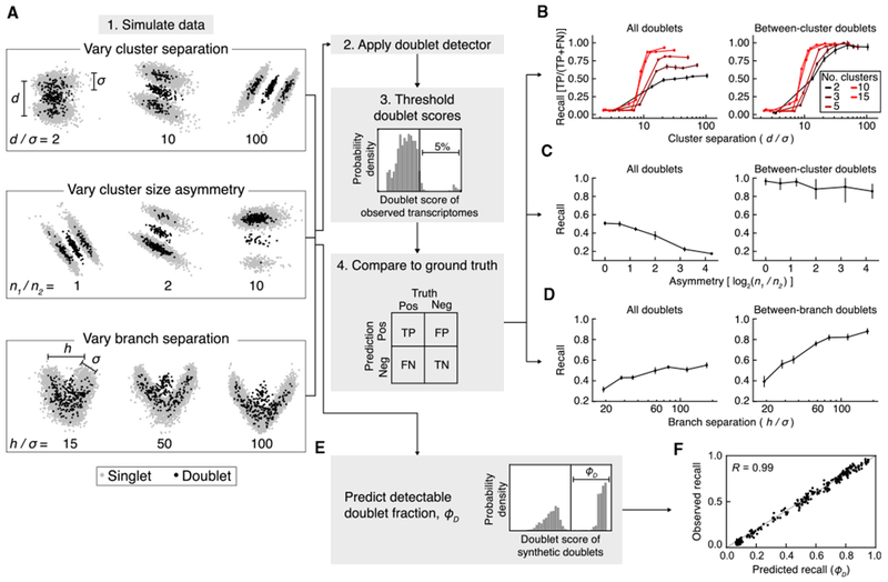
(A) Schematic summary of simulations for testing Scrublet. d, inter-clustervariance; σ, intra-clustervariance; n1, size of larger cluster; n2, size of smaller cluster; h, inter-branch variance. See STAR Methods for full simulation details.
(B) Evaluation of doublet detector performance for varying numbers of clusters and cluster separation. After thresholding doublet scores based on the simulated doublet rate (5%), the recall (true positive rate) was measured using all doublets (left) or between-cluster doublets only (right). Points and error bars are the mean and standard deviation of 10 independent simulations, respectively.
(C) Evaluation of doublet detector performance for two clusters with varying degrees of cluster size asymmetry. Panels and error bars as in (B).
(D) Evaluation of doublet detector performance for a branching continuum with varying degrees of separation between the two branch endpoints. Recall was measured for all doublets (left) and when limiting to doublets formed by cells from opposite branches (right). Error bars as in (B).
(E) Prediction of the detectable doublet fraction, ϕD, using the distribution of scores for the synthetic doublets.
(F) Comparison of predicted ϕD to observed doublet recall for the simulations in (B).
The doublet detector also performed well when predicting doublets in a continuum of cell states: in a simulation of two paths diverging from the same starting state, up to 92% of doublets formed by cells from divergent states (> 10% of the way toward opposite endpoints) were identified at a precision of 98% (Figure 2D). As expected, doublets forming near the point of divergence were poorly identified. In summary, these results illustrate the basic concepts of the classifier in idealized settings with known inputs.
Performance on Dataset #1: Human-Mouse Cell Mixture
We tested the Scrublet on a publicly available dataset consisting of a mixture of human (HEK293T) and mouse (NIH3T3) cells (Figure 3A). This dataset, though not representative of most single-cell experiments, provides a useful test case because the differences between human and mouse genomic sequence provide an independent way to detect doublets (Klein et al., 2015; Macosko et al., 2015). We defined a partial ground truth on doublet identity according to whether a cell barcode associates with transcripts from both species (a doublet) or just one species (Figure 3B). Because doublets arising from the encapsulation of two human or two mouse cells cannot be identified as such, we expected our doublet detector to correctly predict all ground truth labeled doublets, since they arise from distinct human and mouse cell types and should thus be neotypic.
Figure 3. Doublet Prediction for a Mixture of Human and Mouse Cells.
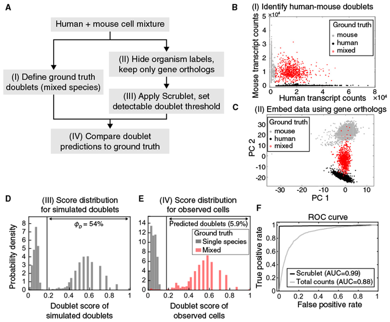
(A) Schematic overview of species mixing experiment.
(B) Identification of mixed-species doublets based on fraction of reads mapping to human or mouse transcriptome.
(C) Principal-component (PC) analysis of single-cell transcriptomes, restricting to human-mouse gene orthologs.
(D) Histogram of doublet scores for simulated doublets. The bimodal distribution reflects the two types of doublets: undetectable intra-species embedded doublets (left peak) and inter-species neotypic doublets (right peak).
(E) Histograms of doublet scores for observed singlets (gray) and doublets (red). See also Figure S2.
(F) Receiver-operator characteristic (ROC) curve for Scrublet and total transcript counts as predictors of inter-species doublets. AUC, area under the curve.
After hiding species labels and restricting to orthologous genes (Figure 3C), Scrublet estimated the detectable doublet fraction at ϕD = 54%, close to the 50% expected for cross-species doublets given equal input of mouse and human cells (Figure 3D). Furthermore, the detector accurately identified human-mouse doublets with a receiver-operator characteristic (ROC) area under the curve (AUC) of 0.99 (recall of 98% of human-mouse doublets with precision of 96%) (Figures 3E, 3F, and S2A), and the overall Scrublet-predicted doublet fraction agreed well with the expected fraction (Table 2). False positives and negatives tended to lie in “boundary states.” Specifically, false negatives (mixed-species doublets incorrectly called as singlets by Scrublet) had lower degrees of species mixing than true positives, while false positives had below-average total transcript counts and lay on the border between the doublet and singlet clusters in PCA space (Figure S2B). Compared to Scrublet, predicting doublets on the basis of total transcript counts was less effective (AUC = 0.88), since the average human cell contained nearly twice as many transcripts as the average mouse cell; to achieve a recall of 90%, the precision dropped to just 15% (Figure 3F).
Table 2.
Scrublet-Predicted and Experimentally Expected Doublet Fractions
| Dataset | Scrublet outputs | Experimental rate | ||||
|---|---|---|---|---|---|---|
| Detected doublets (δ) | Detectable doublet fraction (ϕD) | Overall doublet rate (δ/ϕD) | Overall doublet rate () | Rationale | ||
| Mouse-human (Figure 3) | 5.9% | 54% | 10.9% | ↔ | 11.6% | Using mouse versus human genomes |
| Demuxlet (Figure 4) | 8.1% | 55% | 14.6% | ↔ | 12.2% | Using human SNPs |
| PBMCs (Figure 5B) | 1.8% | 53% | 3.5% | ↔ | 3% | Nominal doublet rate |
| PBMCs (Figure 5C) | 4.1% | 61% | 6.8% | ↔ | 6% | Nominal doublet rate |
| Bone marrow (Figure 6) | 3.6% | 43% | 8.3% | ↔ | 5%–10% | inDrops observed droplet occupancy |
Performance on Dataset #2: Peripheral Blood Cells from Multiple Individuals
To test the doublet detector in a more typical experimental context, we evaluated its performance using a published dataset generated from a mixture of eight genotyped human donors’ mature blood cells (peripheral blood mononuclear cells, PBMCs) (Kang et al., 2018). The authors identified ground truth multiplets as cell barcodes associated with reads containing polymorphisms from more than one individual (Figure 4A). Given that the data represent a similar number of cells from each individual, roughly 7 out of 8 doublets should occur between individuals and can be identified using this approach. Thus, in the ground truth data, we expect at least 12.5% of true doublets to be undetected.
Figure 4. Doublet Prediction for Blood Cells from Eight Genotyped Human Donors.
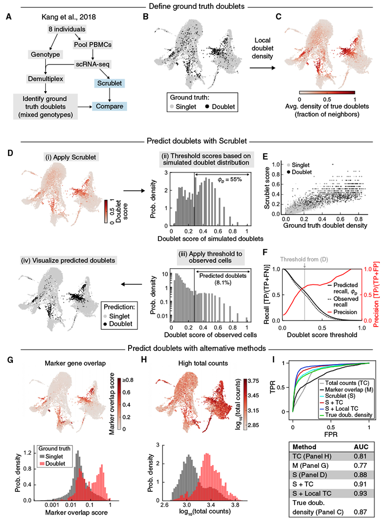
(A) Schematic overview of genotyped cell mixing experiment.
(B) Force-directed graph layout of the profiled cells. Black points indicate ground truth doublets identified by Demuxlet as barcodes associated with polymorphisms from more than one individual (Kang et al., 2018).
(C) Force-directed graph layout of ground truth doublet score, defined as the fraction of a cell’s neighbors that are mixed genotyped doublets.
(D) Application of Scrublet to the transcriptomic data. After calculating doublet scores (i), the histogram of scores for simulated doublets was used to determine a threshold for detection of neotypic doublets (ii). Applying this threshold to observed cell barcodes (iii) yielded doublet predictions for each transcriptome (iv). ϕD, predicted detectable doublet rate. See also Figure S3.
(E) Comparison of Scrublet to the ground truth doublet score, colored by genotype-based doublet labels (singlets, gray; doublets, black).
(F) Comparison of detectable doublet fraction (solid black line) and actual recall (dashed black line) for a range of doublet scorethresholds and the corresponding precision (red line). TP, true positive; FN, false negative; FP, false positive.
(G) Alternative doublet prediction based on co-expression of marker genes of distinct cell types. Upper: force-directed graph layout with cells colored by marker overlap score. Lower: histograms of marker overlap score for ground truth singlets (gray) and doublets (red).
(H) Alternative doublet prediction based total transcript counts. Upper: force-directed graph layout with cells colored by total counts. Lower: histograms of total counts for ground truth singlets (gray) and doublets (red).
(I) ROC curves (upper) and AUC scores (lower) for various doublet prediction methods. “S+TC” and “S+Local TC” are linear combinations of the Scrublet score and total counts or the Scrublet score and total counts relative to neighboring cells, respectively (see STAR Methods for details).
To make use of this orthogonal method for multiplet detection, we compared Scrublet predictions to the ground truth doublets and also generated a “ground truth score” by calculating the fraction of each cell’s neighbors that were mixed genotype doublets (Figures 4B and 4C). Because this score reflects the density of doublets in a region of gene expression space, it is directly comparable to the score computed using Scrublet. We then applied Scrublet to the transcriptomic data (Figure 4D) and compared the Scrublet scores to these ground truth scores (Figure 4E). This comparison showed a fair agreement: 89% of doublets with a high ground truth score (> 0.4) were also identified by Scrublet, with a precision of 77%. The high-scoring cells for both methods co-localized in low-dimensional visualizations of the data (Figures 4B, 4D, and S3A–S3C), with undetected doublets scattered among other cell states. Re-processing the data following removal of true or Scrublet-predicted doublets slightly improved separation of cell types in the 2-D visualization but had little effect on cell clustering, aside from the expected loss of doublet-specific clusters (Figures S3D and S3E). Furthermore, the recall of true doublets was accurately predicted by fD, the detectable doublet fraction as measured by the simulated doublet distribution (Figure 4F). At the selected doublet score threshold, the recall of 49% was in good agreement with the fD of 55%, and this held true across a range of thresholds. This suggests that even though many doublets go undetected, the fraction of identifiable doublets can be accurately estimated. Though the precision was just 66%, this can be explained in part by the imperfect nature of the ground truth labels, since doublets formed by cells from the same individual are undetectable based on genotype alone. Finally, the predicted overall doublet fraction was only slightly higher than the experimentally estimated value (Table 2).
As with the previous dataset, we compared the doublet detector performance to alternative strategies: (1) identifying cells coexpressing curated marker genes of distinct cell types and (2) identifying cells with high total transcript counts. For the former method, we created a list of highly specific marker genes of each cell type in this dataset and then calculated the amount of co-expression of marker genes from different cell types (Figure 4G) to define a “marker co-expression score” (STAR Methods). Of the 773 true doublets correctly identified by Scrublet, 68% also had a high degree of marker gene co-expression. Overall, the “marker co-expression score” did not perform as well as Scrublet (AUC 0.77 versus 0.88) and required significant manual annotation.
For the method relying on high total transcript counts, we found that true doublets did tend to have higher total transcript counts than singlets (AUC = 0.81) (Figures 4H and 4I). Because total counts appeared to be informative and did not require any manual annotation, we created a hybrid predictor by linear combination of each cell’s Scrublet score with its locally normalized total counts (STAR Methods). While this hybrid approach performed better than any other for this particular example (AUC = 0.93) (Figure 4I), its effectiveness could vary across datasets, and it required additional parameter fitting to determine the relative weights of the Scrublet score and total counts score.
Performance on Dataset #3: Peripheral Blood Cells at Multiple Concentrations
In a third test, we turned to a dataset that offers a less direct independent strategy for detecting neotypic doublets: namely, a single sample of PBMCs split and barcoded at two different cell concentrations, yielding either 4,352 (“PBMC-4k”) or 8,391 (“PBMC-8k”) transcriptomes. We reasoned that multiplet-specific cell states should be identifiable as clusters whose relative abundance increases with increasing input cell concentration because, in fully dissociated samples, a doubling of cell concentration doubles the probability of randomly encapsulating two cells into the same droplet. In the PBMC data, states composed uniquely of doublets should double in relative abundance, with cell states that are predominantly singlets decreasing only incrementally (Figure 5A).
Figure 5. Doublet Prediction Using Multiple Concentrations of Blood Cells.
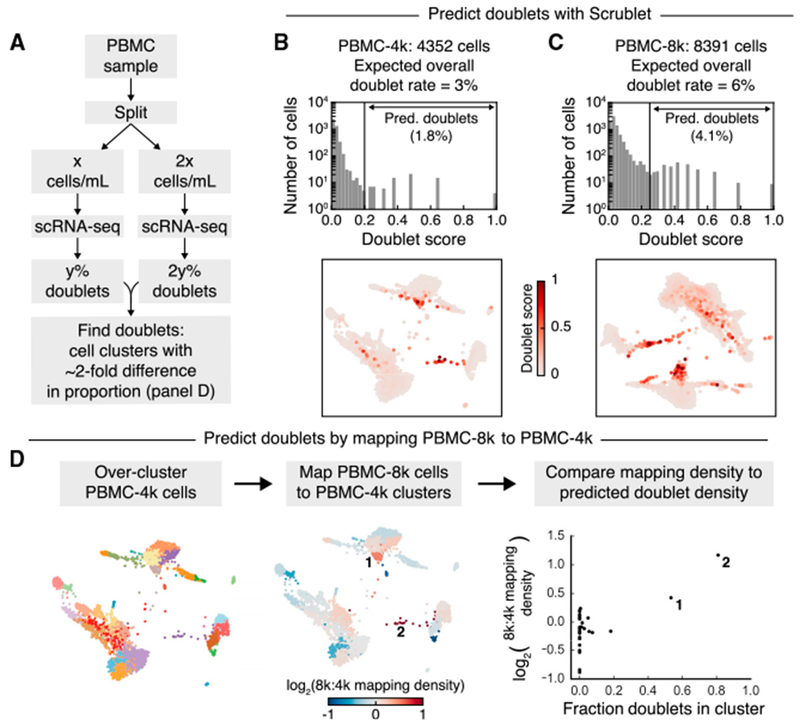
(A) Schematic overview of how multiple concentrations of the same cell sample can be used to identify doublet-specific states.
(B) Scrublet score histogram (upper) and force-directed graph layout (lower) for the low cell concentration (PBMC-4k) sample. See also Figure S4.
(C) Same as (B), but for the high cell concentration (PBMC-8k) sample. See also Figure S4.
(D) Comparison of cluster sizes in PBMC-4k and PBMC-8k samples to identify doublet-specific clusters, which are expected to be disproportionately larger in the PBMC-8k data. After clustering the PBMC-4k cells (left), each PBMC-8k cell was mapped to its most similar PBMC-4k cell, and the proportions of cells from each sample in each cluster were compared (center). This relative cluster abundance was then compared to the Scrublet predictions (right).
As expected, the doublet detector identified roughly twice as many doublets in the PBMC-8k sample (4.1%) as in PBMC-4k (1.8%) (Figures 5B, 5C, and S4A–S4D), and as with the previous datasets, Scrublet’s estimate for the overall doublet fraction was in close agreement with the expected value (Table 2). Furthermore, when we compared the PBMC-8k cells to their most similar PBMC-4k counterparts, the predicted doublet states were present at a higher relative abundance, while singlet states changed little or decreased (Figure 5D). This test again suggests that the doublet detector correctly identifies neotypic doublets.
We used this dataset to demonstrate that removal of doublets can improve the quality of downstream analyses, such as identification of genes expressed in a cell type-specific manner. We identified cell type-specific marker genes in the PBMC-8k dataset before and after excluding Scrublet-predicted doublets. Doublet removal resulted in marked increases in the number of highly specific genes detected for B cells, T cells, and monocytes (Figures S4E and S4F) since many doublets also expressed these genes at relatively high levels.
Prediction of Doublets in a Cell State Continuum
The above examples demonstrate Scrublet’s ability to correctly identify neotypic doublets from datasets consisting of distinct cell types. In a final example, we applied it to a continuum of cell states by analyzing transcriptomes of KIT+ hematopoietic progenitors from the mouse bone marrow (Tusi et al., 2018) (Figure 6A). These cells form a continuum from multipotent progenitors to unilineage committed cells. Several groups of doublets were readily distinguishable (Figures 6B, 6C, and S5) and formed “bridges” between different committed progenitor types. Here, we lack a ground truth for confirming the identity of the doublets, but since such bridges are inconsistent with our current understanding of hematopoiesis, it is likely that our doublet detector is correct in identifying them.
Figure 6. Prediction of Doublets in a Continuum of Differentiating Hematopoietic Progenitors.
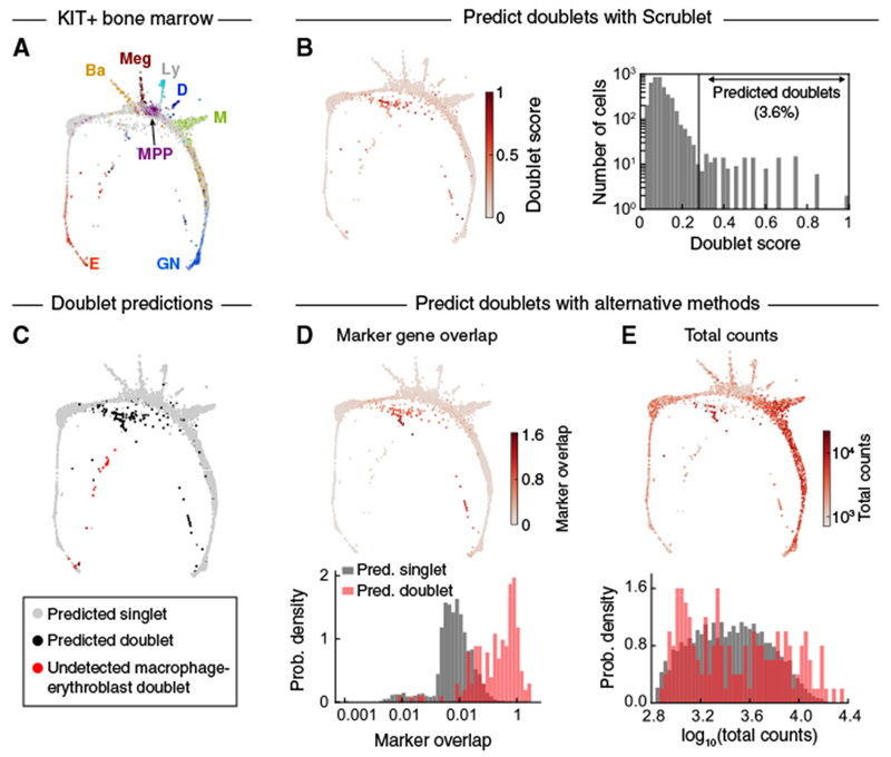
(A) Force-directed graph layout of KIT+ mouse bone marrow cells profiled by scRNA-seq. Cells are colored by expression of established marker genes. E, erythroid; Ba, basophil/mast cell; Meg, megakaryocyte; MPP, multipotent progenitor; Ly, lymphoid; D, dendritic cell; M, monocyte; GN, granulocytic neutrophil. Adapted from Tusi et al., 2018.
(B) Force-directed graph layout colored by Scrublet score (left) and histogram of Scrublet scores (right). See also Figure S5.
(C) Predicted doublets localized on force-directed graph layout. Gray, predicted singlets; black, Scrublet-predicted doublets; red, likely erythroblast-macrophage doublets (C1qa+ Hba-a1+), undetected by Scrublet due to absence of macrophage singlets in the KIT+ data.
(D) Alternative doublet prediction based on coexpression of marker genes of distinct cell types. Upper: force-directed graph layout with cells colored by marker overlap score. Lower: histograms of marker overlap score for Scrublet-predicted singlets (gray) and doublets (red).
(E) Alternative doublet prediction based on total transcript counts. Upper: force-directed graph layout with cells colored by total counts. Lower: histograms of total counts score for Scrublet-predicted singlets (gray) and doublets (red).
We again compared Scrublet to other approaches based on marker genes or total counts. As before, predicted doublets consistently expressed combinations of marker genes for distinct maturing progenitor states (Figure 6D), while only some predicted doublets had above average total transcript counts (Figure 6E).
This dataset was also instructive in highlighting a shortcoming of our approach when one of its assumptions is violated. Namely, Scrublet can detect cell aggregate doublets only if both parent cell types are observed as singlets elsewhere in the dataset. Through manual curation, we identified a small group of transcriptomes co-expressing markers of erythroblasts and mature macrophages (Figure 6C). Macrophages and KIT+ erythroblasts are known to physically associate in the bone marrow in erythroblastic islands (Manwani and Bieker, 2008) and have been observed in other scRNA-seq datasets (Grun et al., 2016). Since macrophages do not express the cell surface receptor KIT, used for cell purification in this experiment, they appear only in the form of doublets in this dataset. Unfortunately, such aggregates might confound other methods for doublet detection, including all of the experimental methods in Table 1. They may, however, be identifiable by combining multiple datasets in orderto provide the full set of singlet states for Scrublet.
DISCUSSION
We proposed and tested a classification scheme for cell multiplets, focusing on cell doublets, as these are expected to form the majority of multiplets in all but specialized cases. The classifier is trained using the data itself and reasonable assumptions about the structure of gene expression space. The application to simulated data and then to four empirical datasets demonstrates that the approach can accurately identify doublets formed by cells from distinct states, as assessed by formal estimates of recall and precision where possible. The cell transcriptomes that scored as doublets with the highest confidence were also those found after manual curation of the data to co-express marker genes of distinct cell states. The classification approach outper-formed manual curation and simple total counts-based approaches, although it benefitted from being combined with total counts information. We demonstrated the practical benefits of doublet removal in removing artifactual states and in improving the signal-to-noise in the expression of cell type-specific genes.
Although the method appears to perform well, its underlying assumptions do impose some limitations. First, the method assumes that multiplets are rare. This is required (1) to justify the study of doublets rather than all multiplets and (2) for the doublets simulated by the classifier to overwhelmingly reflect doublet states rather than higher-order states. Second, the method strictly requires that every cell state contributing to a doublet also be represented as a singlet state in the dataset. If a particular singlet cell state is excluded experimentally, it trivially cannot be detected as part of a multiplet state, because the missing parent state does not contribute to the simulated doublet pool used for doublet classification. This limitation could be appreciated in the final dataset, from cells purified conditional on expression of a cell surface protein, KIT. We found that cell doublets resulting from incomplete dissociation of a KIT+ erythroid cell and a KIT-macrophage could not be detected by the classifier because no singlet macrophage state was present in the dataset. An extension of this limitation is that the method could underperform if cell clumps with a stereotyped composition occurred in a sample. Scrublet performs best for doublets resulting from random co-encapsulation because the frequency of such doublet states can be predicted by the frequency of singlet states. Doublets from incomplete dissociation can still be effectively detected provided that they are rare and that the singlet states are well represented in the data.
A third limitation of the approach is its sensitivity to the structure of the single-cell state manifold. Scrublet performs best in identifying doublets formed between distinct parent states. This limitation is quantified for any given dataset by the calculated detectable doublet fraction, ϕD, which is expected to be high if singlet states are distributed among many discrete, well-separated states; it is only 50% if cells form two discrete and equal-sized clusters, and it can be lower than 50% for complex continuum manifolds. Countering this shortcoming is the notion that rare doublet states are only important to exclude if they form novel features on a cell state manifold, which would in turn make them detectable using the proposed approach. Therefore, the doublet detector provides a useful tool both for estimating the potential impact of doublets on downstream hypothesis generation through the magnitude of fD and for identifying bona fide doublet states for exclusion.
STAR★METHODS
CONTACT FOR REAGENT AND RESOURCE SHARING
Further information and requests for resources should be directed to and will be fulfilled by the Lead Contact, Allon Klein (allon_klein@ hms.harvard.edu).
METHOD DETAILS
The Scrublet Algorithm
A formal basis for the doublet classifier is provided in the “Scrublet Theory” section, below.
Definitions
For clarity, we use the term “singlet” to refer to a transcriptome of a single cell and “doublet” to refer to a merged transcriptome of two cells. The majority of observed transcriptomes are expected to be singlets.
General Approach
Starting with a raw counts matrix, X, where xi,j is the number of detected transcripts of gene j in cell i,
Pre-filter cell barcodes to exclude background, typically barcodes with insufficient total transcripts detected.
Simulate doublets by combining the counts from random pairs of cells: the counts for gene j in doublet i with parent cells a and b is yi,j = xa,j + xb,j.
Build a k-nearest-neighbor (KNN) classifier, labeling observed cells as 0 and simulated doublets as 1. In detail, construct a KNN graph using the union of observed cells and simulated doublets and calculate the doublet score as the fraction of neighbors that are simulated doublets.
Remove likely doublets by thresholding the doublet scores or by clustering observed cells and identifying clusters with uniformly high scores.
Detailed Method
Throughout this paper and in the code provided online at github.com/AllonKleinLab/scrublet, we implement the doublet detector as described in the following sections. However, our online code also allows for arbitrary preprocessing, enabling users to apply their preferred methods for gene filtering, normalization, dimensionality reduction, etc., prior to running the core doublet detector code.
Default Preprocessing
Starting with a background-filtered, UMI-based counts matrix for the observed cells, we perform normalization, gene filtering, and principal components analysis (PCA):
Normalize each cell by its total counts, setting the post-normalization total to the average total of all cells. That is, the normalized counts for gene j in cell i were calculated from the raw counts, xi,j, as , where Xi = ∑jxi,j and is the average Xi over all cells.
Identify highly variable genes, keeping genes with ≥ng counts in ≥nc cells and in the top qth percentile of most variable genes, as measured by V-score (baseline-corrected Fano factor) (Klein et al., 2015). Default values are ng = 3, nc = 3, and q = 85 (i.e., the 15% most variable genes).
Using the genes identified in step 2, Z-score standardize the data such that each gene has mean of zero and standard deviation of unity. Store the means and standard deviations for downstream scaling of the counts for simulated doublets (below).
Run PCA (unweighted). Store the eigenvectors (gene loadings) for transformation of simulated doublets (below).
Note that for three of the datasets (“human-mouse”, “Demuxlet PBMCs”, and “PBMCs at multiple concentrations”), we used a variant of steps 3 and 4 that maintains the sparse nature of the data and reduces computational costs, as this will likely be important for dealing with increasingly large single-cell datasets. Namely, in step 3 the data were standardized but not mean-centered, and for step 4 truncated singular value decomposition (SVD) was used in place of PCA. These alternative options are available in the pre-processing pipeline implemented in our online code.
Doublet Simulation
Doublets are simulated by adding the unnormalized counts from randomly sampled observed transcriptomes. Doublet transcriptomes are then transformed into the same PCA space as the observed transcriptomes through the following steps:
Normalize gene expression for each simulated doublet (same as step 1 of “Preprocessing”, above).
Apply the gene filter from step 2 of “Preprocessing”.
Standardize the simulated data using the same gene means and standard deviations as measured in the observed transcriptomes (step 3 of “Preprocessing”), i.e., rather than re-calculating the mean and standard deviation for each gene based on the simulated data, simply subtract the gene’s observed mean and divide by its observed standard deviation.
Apply the eigenvectors from step 4 of “Preprocessing” to embed simulated doublets in the same PCA space as the observed transcriptomes.
KNN Classifier
For the default preprocessing, a KNN graph is built using Euclidean distance in the combined PCA embedding of the observed and simulated cells. Scrublet further allows for constructing a KNN graph in a user-defined embedding, in place of PCA. To set the number of neighbors, Scrublet accepts a parameter k for the average number of observed transcriptome neighbors, and a parameter r for the ratio of the number of simulated doublets to observed transcriptomes. The adjusted number of graph neighbors, kadj = round(k·(1+r)), is used to construct the graph. We have found that setting and r≥2 works well. For large datasets, an approximate nearest neighbor algorithm is used for graph construction, as this dramatically improves speed with little cost in accuracy (Bernhardsson, 2013).
Next, and , the doublet scores for the observed transcriptomes {xi} and simulated doublets {yi}, respectively, are calculated by finding the fraction of each transcriptome’s neighbors that are simulated doublets and calculating the Bayesian Likelihood derived in the “Scrublet Theory” section, below. For transcriptome i with kd(i) simulated doublet neighbors, the doublet score is
where
and is the estimated doublet rate (i.e., fraction of observed transcriptomes that are doublets), which is provided as input to the Scrublet classifier.
A standard error is also calculated for , (see “Scrublet Theory”, below):
where
and is the uncertainty in the estimated overall doublet rate, which additionally is provided as input to the Scrublet classifier.
Setting the Doublet Score Threshold
After computing the doublet scores and , a threshold θ is set based on the distribution of , and observed transcriptomes with are predicted as doublets. In all of the presented examples, the distribution of was bimodal, reflecting the partitioning of doublets into embedded and neotypic types. The threshold was set by eye to lie between the two peaks of the histogram of . We also provide a method for automatic threshold detection using the skimage.filters.threshold_minimum function from the Python package scikit-image, though we still recommend visual inspection of the histogram of to confirm the threshold has been set in a reasonable location.
After setting a threshold, a measure of confidence in the doublet predictions is provided by a z-score,
Recommended Self-Consistency Tests
While the Scrublet package may be used as-is, we recommend two self-consistency tests:
Confirm that the distribution of likelihoods of simulated doublets, , is bimodal.
We expect the fraction of observed transcriptomes predicted to be doublets, δ, to roughly equal .
If the first condition is not satisfied, the choice of may be incorrect; if the second condition is not satisfied, then the choice of θ may be incorrect. Alternatively, the assumptions required for the classifier may be violated.
Scrublet Theory
In this section we offer a formal definition for “embedded” and “neotypic” multiplets, provide a derivation of the doublet Likelihood, motivate the method for Likelihood threshold choice for the Scrublet classifier, and define the “detectable doublet fraction”. Equations 7, 8, and 10 derived below define key outputs of the Scrublet classifier and are referred to in the “Scrublet algorithm” section, above.
Defining Neotypic and Embedded Multiplets
Probability Distributions of Sampled Transcriptomes.
Consider a set of observed transcriptomes, , with ui, = (ui1,…,uiN) being a vector of the expression values of N genes for the i-th transcriptome. Two probability density functions and respectively describe the distribution of singlets and doublets from which {ui} are sampled. Some observed transcriptomes ui correspond to singlet cells sampled from , and others correspond to doublets sampled from . If ρ is the fraction of sampled transcriptomes that are doublets, then the observed transcriptomes are sampled from the probability density function .
The processing of single-cell data involves one or more steps of normalization, gene selection and/or embedding that collectively define a map from the original gene expression space to a new space Ω that is , or in the case of additional discrete cluster assignment, Ω is (possibly with M = 0 if only discrete clustering is performed). In what follows, the results hold for any choice of map f. We define f to generally encompass methods for single-cell data analysis including, for example, total count normalization, selection of a subset of genes for downstream analysis, principal component analysis, methods for non-linear embedding, a possible adoption of a cosine distance, assignment of cells to discrete clusters, and so on. Under the action of this map, the sampled transcriptomes are xi = f(ui), and one generates probability densities of singlets and doublets in the mapped spaces, PS(x) and PD(x), and the observed transcriptomes are distributed as,
| (Equation 1) |
We denote these distributions without the “~” sign to distinguish them from the original probability densities in .
Neotypic versus Embedded Doublets.
A doublet with transcriptome u, mapped to x = f(u)∈Ω, can be considered “embedded” among singlets if , i.e., if it occupies a region of Ω that is overwhelmingly occupied by singlets. Conversely, a doublet can be considered “neotypic” if , i.e., if it occupies a region of U that is overwhelmingly occupied by sampled doublets. Finally, if , then a doublet occupies a region occupied by comparable numbers of singlets and doublets, and it is neither neotypic nor embedded in the qualitative sense proposed in this paper. In such cases, the doublets do not generate qualitatively new cell states, but they significantly perturb existing cell states and may be considered to be “perturbative” doublets. In summary:
Thus, “neotypic” and “embedded” doublets can be considered as limiting cases. When doublets are rare (ρ ≪ 1), we propose that most doublets occupy regions of Ω that are embedded or neotypic. For this reason, the classification is a useful one. One can however imagine specialized cases where many doublets are perturbative (as per the above classification), for example if ρ is not small.
The Operational Nature of Doublet Errors.
Because the map f is not isomorphic (e.g., since M<N), it will not preserve the ratios of singlet and doublet distributions, i.e., in general . This means that a multiplet state u could appear embedded in one map Ω1, but neotypic in another map Ω2. This is easy to appreciate: for example, if analysis is restricted to one subset of genes, then some doublets may be neotypic, while restriction to another subset of genes might cause the same doublets to be embedded.
The operational dependence of doublet classification on the choice of map f means that the nature of doublet errors cannot be considered to be immutable properties of the doublets. A doublet error analysis may need to be carried out for each choice of data analysis. In the “Detectable doublet fraction” section, below, we revisit this ambiguity when considering the theoretical detectable doublet fraction.
The Doublet Likelihood
In the following we derive the Likelihood that a mapped transcriptome x = f(u)∈Ω is a doublet, in the limiting case where doublets are rare (ρ ≪ 1). The doublet Likelihood serves as a basis for classification.
As will become clear, is sensitive to our prior belief in the doublet rate ρ. It will be useful to distinguish between the true doublet rate, ρ, and our prior belief in its value, which we denote . Because can be inaccurate, we do not classify doublets directly based on an invariant threshold , but instead estimate a threshold value θ in a manner that is not sensitive to . For clarity, the table below summarizes the symbols introduced in this derivation.
Summary of symbols
| u | Measured cell transcriptome () |
| Ω | Embedding space to which u is mapped |
| X∈Ω | Cell transcriptome after dimensionality reduction |
| Ps(x) | Probability density of singlets (in Ω) |
| PD(x) | Probability density of true doublets (in Ω) |
| P′D(x) | Probability density of simulated doublets (in Ω) |
| P obs (x) | Probability density of observed transcriptomes (in Ω) |
| ρ | Fraction of observed transcriptomes that are doublets |
| Prior belief in the value of ρ | |
| Mobs | Total number observed transcriptomes |
| M D | Total number simulated doublets |
| r | MD/Mobs |
| k | Number of nearest neighbors for KNN classification |
| k d | Number of nearest neighbors to x that are simulated doublets |
| k obs | Number of nearest neighbors to x that are observed transcriptomes |
| q(x) | The binomial proportion of nearest neighbors that are simulated doublets |
| The Likelihood that a transcriptome x is a doublet | |
| 〈·〉 | Expectation value of an estimator |
| SE[·] | The standard error of the estimator |
Relationships between probability densities.
To develop a doublet classifier for a point x∈Ω, the Bayesian approach is to assign x as a doublet if , or a singlet otherwise. Though PS and PD are not known, they can be approximated. From Equation 1, in the limit ρ ≪ 1 the probability density of observed transcriptomes approximates that of singlets:
The approximation of the doublet distribution is similar: if sampled uniformly, then true doublets are a convolution of singlets, i.e., , while simulated doublets, with probability density P′U, are generated by combining transcriptomes sampled from , i.e., a convolution of observed transcriptomes . Therefore, P′D(x) is approximately the doublet probability density, with an error of order ρ:
The Approximate Doublet Likelihood.
From Bayes’ theorem,
From Equation 1 and the above approximations, we can rewrite in terms of measured distributions, discarding terms of higher order in ρ and :
| (Equation 2) |
In the last line, to avoid having a Likelihood greater than one, we introduced a small correction of order . This form is a perfect Bayesian Likelihood under the approximation that P′D=PD and Pobs=PS.
Theoretical Binomial Proportion.
We construct a nearest-neighbor classifier with a total number of MD simulated doublets, and a total number of Mobs observed transcriptomes. Let r = MD/Mobs. The theoretical probability of randomly sampling a simulated doublet in the neighborhood of x is then
| (Equation 3) |
It can be seen from Equations 1 and 2 that is a monotonic function of q:
| (Equation 4) |
Estimator of the Binomial Proportion.
For any single transcriptome, we can estimate the binomial proportion q(x)from the KNN classifier output, which reports on the number kd of simulated doublets that are found to be nearest neighbors of x out of the k nearest neighbors. For brevity, we denote q(x) as q. With a uniform prior on q∈[0,1], the posterior distribution of q follows a Beta distribution with expectation value,
| (Equation 5) |
and standard error,
| (Equation 6) |
Estimator of the Doublet Likelihood.
From Equations 4, 5, and 6, one can calculate the Likelihood of a sampled transcriptome x being a doublet. It is additionally useful to obtain a measure of confidence in our estimator of . Assuming small errors in q, the estimator of the doublet Likelihood and its standard error are
| (Equation 7) |
and,
| (Equation 8) |
These two expressions are central results calculated by the Scrublet pipeline, as described in the “Scrublet algorithm” section, above. The quantity , introduced here, provides a measure of uncertainty in the doublet rate . To obtain the last expression, we write down the error propagation formula,
| (Equation 9) |
and then calculate the relevant derivatives from Equation 4,
and
These expressions together give Equation 8.
Thresholding the Doublet Likelihood
In principle, the doublet likelihood alone could be used to decide on which cells are putative doublets: if , call a cell a doublet. The confidence in the call is simply the value of itself.
However, the doublet likelihood is sensitive to the prior guess, , on the fraction of observed transcriptomes that are doublets. In practice is known roughly, but it is easy to be off by several-fold from its true value ρ. Though uncertainty in is already used to estimate the error in in Equation 8, we should ideally look for a method of doublet classification that is not sensitive to .
To do this, we treat as a feature on which to perform classification, rather than as a strict posterior Bayesian probability. From Equation 4 one can see that the value of is then a parameter that monotonically rescales , i.e., preserving the ordering of all cells.
Practically, if is larger than a threshold value θ, we call it a doublet. The confidence in the call is reflected by a z-score,
| (Equation 10) |
calculated from Equations 7 and 8. z(x) is provided as an output of the Scrublet pipeline for each transcriptome.
To set the threshold value θ, we rely on our initial guess that doublets are overwhelmingly neotypic or embedded, with few perturbing doublets (see “Defining neotypic and embedded multiplets”, above). Defining {yi = f(ui)}∈Ω as embedded transcriptomes of simulated doublets only, we should expect values of to be bimodally distributed. We can then set the threshold θ by looking for a minimum between two modes (high and low) in the distribution of doublet Likelihoods . The Scrublet pipeline offers an automated procedure for thresholding. Practically, however, it is advised for self-consistency to inspect the distribution of to confirm that it is indeed bimodal.
The success of this approach in rendering the Scrublet result insensitive to the value of the input parameter is demonstrated in Figure S3F, which plots the detectable doublet fraction ϕD (see next section) for different guesses for , and in Figure S3G, which shows how the final doublet calls change with the value of . Changing also does not affect the AUC, because the rank ordering of doublet scores is independent of .
The Detectable Doublet Fraction
Ideally, one would wish to define a theoretical detectable doublet fraction, as the fraction of doublets that could be distinguished from singlets using any method only has access to empirical transcriptomic data, e.g., by finding the optimal map f(u) that maximally separately doublets from singlets.
We do not know how to estimate , or even whether it is knowable. Instead, we define an operational detectable doublet fraction, ϕD, for a given choice of dimensionality reduction map f and a chosen threshold, θ, as
where H(x) is the indicator function (H(x) = 1 for x≥0, 1 otherwise). The value of ϕD can be calculated as the fraction of simulated doublets correctly detected by the classifier.
Note that ϕD is not equivalent to the fraction of observed transcriptomes determined to be doublets,
We observe that if is correctly estimated, then , i.e., the fraction of all doublets that are detected in the data set should approximately equal the operationally defined fraction ϕD.
Testing Scrublet
Splatter Simulations
We used the Splatter R package (v1.0.3) (Zappia et al., 2017) to simulate ground truth data for testing the doublet detector. For each set of parameters, we simulated 10 replicates with 5000 cells and 2000 genes, using default parameters except where noted below. Doublets were simulated at a rate of 5% by randomly sampling (without replacement) pairs of cells and summing their counts; cells used to generate doublets were then removed from the data. The table below summarizes the conditions simulated for Figure 2.
Splatter simulation parameters
| Panel | Number of groups | Group1 size/Group2 size | Splatter parameter “method” | Splatter parameter “mean.shape” | Splatter parameter “de.prob” |
|---|---|---|---|---|---|
| B | 2, 3, 5, 10, 15 | n/a (all uniform) | groups | 0.5 | 0.005, 0.01, 0.02, 0.03, 0.04, 0.05, 0.1 |
| C | 2 | 1, 1.5, 2.3, 4, 9, 19 | groups | 0.5 | 0.05 |
| D | 2 | 1 | Path | 0.5 | 0.01, 0.02, 0.05, 0.1, 0.15, 0.25, 0.4 |
Prior to predicting doublets, PCA was run using genes with at least 3 counts in at least 3 cells. For Figures 2B and 2C, we used all PCs with eigenvalues that were at least 20% of the maximum eigenvalue. For Figure 2D, the top 4 PCs were used for all conditions. The doublet detector was run using k = 40, r = 5, and .
To determine the overall recall (; TP, true positives; FN, false negatives), we set a doublet score threshold based on the simulated doublet rate of 5%; that is, cells with doublet scores in 95th percentile or above were labeled as predicted doublets. Thus, the precision (; FP, false positives) is equal to the recall. The same procedure was used to measure the recall for between-cluster doublets, restricting to doublets formed by cells from different groups. For the branching continuum simulation, between-branch doublets were defined as doublets formed by cells on opposite branches and with Splatter pseudotime >10%.
Human-Mouse Dataset
Pre-processing and Doublet Detector Parameters.
Separate pre-filtered counts matrices for human and mouse genes were downloaded from 10X Genomics (support.10xgenomics.com/single-cell-gene-expression/datasets/2.1.0/hgmm_12k), along with species assignments for each barcode (6,164 human cells, 5,915 mouse cells, and 741 mixed human/mouse multiplets). To create a single counts matrix blind to the species of origin, each cell’s UMI counts for genes with identical mouse and human names (n = 15,642 genes) were added together, and all other genes were excluded. For truncated SVD, we used the top 20% most highly variable genes with ≥3 counts in ≥5 cells (n=2,372 genes) and kept the first two PCs. Scrublet was run using k = 50, r = 10, and (twice the observed rate of human-mouse doublets). To classify cells as singlets or doublets, a threshold was set by eye using the histogram of doublet scores for simulated doublets (Figure 3D).
Demuxlet PBMC Dataset
Pre-processing and Doublet Detector Parameters.
A filtered counts matrix (14,619 cells and 35,635 genes) was downloaded from GEO (GEO: GSM2560248), and demuxlet singlet/doublet calls were obtained from the paper’s GitHub page (github.com/yelabucsf/demuxlet_paper_code). For truncated SVD, we used the top 25% most highly variable genes with ≥2 counts in ≥3 cells (n=3,197 genes) and kept the first 25 PCs. Scrublet was run using k = 50, r = 5, and (the observed doublet rate). To classify cells as singlets or doublets, a threshold was set by eye using the histogram of doublet scores for simulated doublets (Figure 4D).
Ground Truth Doublet Score.
The ground truth doublet score was created by building a KNN graph (k =35) using the observed cells and calculating the fraction of each cell’s neighbors labeled as doublets by demuxlet.
2-D Visualization.
Transcriptomes were visualized using a force-directed layout of the four-nearest-neighbor graph of observed cells, where neighbors were identified using Euclidean distance in PC space. Alternative visualizations were generated from the PCA coordinates using t-distributed stochastic neighbor embedding (t-SNE) (van der Maaten, 2014) with perplexity=30 and angle=0.5 and Uniform Manifold Approximation and Projection (UMAP) (McInnes et al., 2018) using 10 nearest neighbors.
Marker Gene Co-Expression Score.
The marker gene co-expression score was created by identifying highly specific marker genes for each cell type, smoothing expression of these genes over the four-nearest-neighbor graph (see “Graph-based smoothing”, below), and summing the products of pairs of non-overlapping marker genes. In detail, we combined the following pairs of marker genes:
T-cell and NK cell: CD27 × SH2D1B, CD27 × IGFBP7, CD27 × KLRF1
T-cell and B-cell: CD27 × BANK1, CD2 7 × BLK, CD27 × MS4A1
T-cell and monocyte: CD27 × CST3
B-cell and NK cell: BANK1 × SH2D1B
Letting be the smoothed, normalized gene expression of gene j in cell i, the composite score for a pair of genes a and b is
For a given cell type pair p with gene pairs 1,2,…n, the marker gene overlap score for cell i is defined as
And the composite marker gene overlap score for all cell type combinations (as shown in Figure 4G) is ∑pMi,p.
Hybrid Doublet Score (Scrublet + total counts).
For this dataset, we also tested whether combining total counts information with the Scrublet score would improve doublet classification, e.g., by enabling detection of embedded doublets (Figure 4I). In both versions described below, the parameters (relative weights of Scrublet and total counts-based scores) were fit to maximize the AUC.
We tested a simple linear combination of Scrublet and total counts .
We created a “local total counts” (Ci) score, defined as a cell’s total counts divided by the average total counts of its simulated doublet neighbors, and combined it with Scrublet: .
PBMCs at Multiple Concentrations
Pre-processing and Doublet Detector Parameters.
Filtered counts matrices were downloaded from 10X Genomics (PBMC-4k: support.10xgenomics.com/single-cell-gene-expression/datasets/2.1.0/pbmc4k; PBMC-8k: support.10xgenomics.com/single-cell-gene-expression/datasets/2.1.0/pbmc8k). For truncated SVD, we used the top 15% most highly variable genes with ≥3 counts in ≥3 cells (PBMC-4k, n=1,129 genes; PBMC-8k, n=1,307 genes) and kept the first 30 PCs. Scrublet was run using k = 50, r =5, and (PBMC-4k) or (PBMC-8k), based on the expected doublet rates (support.10xgenomics.com/permalink/3vzDu3zQjY0o2AqkkkI4CC). To classify cells as singlets or doublets, a threshold was set by eye using the histogram of doublet scores for simulated doublets.
2-D Visualization.
Transcriptomes were visualized using a force-directed layout of the four-nearest-neighbor graph of observed cells, where neighbors were identified using Euclidean distance in PC space. Alternative visualizations were generated from the PCA coordinates t-SNE with perplexity=30 and angle=0.5 and UMAP using 10 nearest neighbors.
Mapping PBMC-8k to PBMC-4k.
To map the PBMC-8k data to the PBMC-4k data, we TPM-normalized both datasets, ran PCA on the PBMC-4k cells, and used the same eigenvectors to transform the PBMC-8k data. The PBMC-4k cells were clustered using spectral clustering of the four-nearest-neighbor graph with 30 clusters. We then mapped each PBMC-8k cell to its nearest PBMC-4k cell (Euclidean distance) and calculated the number of PBMC-8k cells mapping to each PBMC-4k cluster. In Figure 5D, we present the relative number of PBMC-8k cells per cluster; that is, if nj is the number of PBMC-8k cells mapping to cluster j and N4k and N8k are the total number of PBMC-4k and PBMC-8k cells, then the relative mapping frequency for cluster j is .
Identifying Marker Genes.
The PBMC-8k dataset was used as an example to show that removing doublets can improve detection of cell type-specific marker genes (Figures S4E and S4F). Our goal was to identify highly specific marker genes at the level of major cell types, so we first used Louvain clustering (Blondel et al., 2008) to make an initial set of clusters and then merged clusters manually to give one cluster per cell type (B-cells, T-cells, natural killer cells, monocytes, dendritic cells, and two doublet-specific clusters). For each cluster, we tested genes expressed in >5% of cells in the cluster. For a gene to be considered a marker, there were two requirements. First, it had to be significantly differentially expressed between cells within the cluster and cells outside the cluster, using a Wilcoxon rank-sum test (scipy.stats.ranksums) with a p-value<0.05 after Benjamini-Hochberg correction for multiple hypothesis testing (Benjamini and Hochberg, 1995). Second, the average expression (1+transcripts per million, TPM) within the cluster had to be two-fold higher than in the cluster with the next-highest average expression (i.e., [1 +TPMwithin cluster] / [1 +TPM2nd-max cluster] > 2). This test was run before and after removal of Scrublet-predicted doublets.
Hematopoietic Progenitor Dataset
Pre-processing and Doublet Detector Parameters.
The raw counts matrix was downloaded from GEO (GEO: GSM2388072). Restricting to cells from library batches 2, 3, and 4, we also excluded cells with fewer than 700 total counts or with >15% mitochondrial gene counts (n=4,273 cells final). For PCA, we filtered genes using the same method as the original paper (Tusi et al., 2018), keeping genes with mean expression >0.05 counts and a coefficient of variation >2 (n=7,255 genes), and kept the first 40 PCs. Scrublet was run using k = 50, r = 5, and . To classify cells as singlets or doublets, a threshold was set by eye using the histogram of doublet scores for simulated doublets. After removing high-scoring cells (Scrublet score >0.28, n=146 cells), we re-ran Scrublet and observed additional likely doublets that had been residing at the core of a dense doublet cluster in the original data (round 2 Scrublet score >0.28, n=34 cells). Following removal of these cells, a third round of Scrublet yielded no additional likely doublets.
2-D Visualization.
Transcriptomes were visualized using the force-directed graph layout appearing in the original publication, with minor modifications. Because the published plot was generated after removing doublets, we added doublets back to the visualization by building a KNN graph (k=4) with all transcriptomes (filtered as described above) and running a force-directed graph layout with the positions of the original cells fixed in place, allowing the remaining cells to relax. Alternative visualizations were generated from the PCA coordinates t-SNE with perplexity=30 and angle=0.5 and UMAP using 10 nearest neighbors.
Marker Gene Co-expression Score.
The marker gene co-expression score was created by identifying highly specific marker genes for each cell type, smoothing expression of these genes over the four-nearest-neighbor graph (see “Graph-based smoothing”, below), and summing the products of pairs of non-overlapping marker genes. The combined marker overlap score was calculated as described in the “Demuxlet PBMC dataset” section, above.
We combined the following pairs of marker genes to identify doublets that were also detected by Scrublet (Figure 6D):
Early erythroid and early neutrophil: Car1 × Mpo
Early erythroid and late neutrophil: Car1 × Ngp
MPP and late neutrophil: Cd34 × Ngp
And to identify macrophage-erythroblast doublets (n=37 cells) undetected by Scrublet (Figure 6C):
C1qa × Hba-a1
Graph-Based Smoothing
We used a diffusion-based method to smooth data over the KNN graph for the purposes of finding overlapping marker gene expression (Figures 4F and 6D). In detail, we computed the smoothing operator S = expm(−βL), where L is the Laplacian matrix of the KNN graph, β is the strength of smoothing (β =1 throughout), and expm is the matrix exponential (scipy.linalg.expm from the SciPy Python package). If X* is the smoothed version of gene expression vector X, then X* = SX.
Scalability Testing
To test how Scrublet scales with cell number as shown in Figure S1, we timed our implementation for different numbers of cells, using a computer with a 2.1 GHz processor and 48 GB of memory, though this amount of memory was only necessary for the largest datasets. Timing was broken into stages: preprocessing and embedding, doublet simulation, and the nearest neighbor classifier. To generate datasets of different sizes (n=10 replicates per dataset size), we randomly sampled the desired number of cells from the Demuxlet PBMC dataset, and for each cell randomly sampled from its transcripts with replacement. Scrublet was then run on the randomly sampled data, using, r = 2, , and .
DATA AND SOFTWARE AVAILABILITY
Python code and examples implementing the doublet detector are provided at github.com/AllonKleinLab/scrublet. Scrublet has also been incorporated into SPRING (kleintools.hms.harvard.edu/tools/spring.html), an interactive tool for single-cell data exploration (Weinreb et al., 2018).
Supplementary Material
KEY RESOURCES TABLE
Highlights.
We define two multiplet errors in single-cell RNA-seq data: “embedded” and “neotypic”
Neotypic errors can lead to misidentification of cell types or transitional states
Scrublet code identifies neotypic doublets and predicts the overall doublet rate
The algorithm is tested against several experimental methods for labeling multiplets
ACKNOWLEDGMENTS
This work was supported by NIH grants 1R01HL141402 and 5R33CA212697 and an Edward Mallinckrodt, Jr. Foundation grant. We thank James Briggs for insightful discussion in conceptualizing the approach.
Footnotes
SUPPLEMENTAL INFORMATION
Supplemental Information can be found with this article online at https://doi.org/10.1016/j.cels.2018.11.005.
DECLARATION OF INTERESTS
A.M.K. is a co-founder of 1Cell-Bio.
REFERENCES
- Adamson B, Norman TM, Jost M, Cho MY, Nunez JK, Chen Y, Villalta JE, Gilbert LA, Horlbeck MA, Hein MY, et al. (2016). A multi-plexed single-cell CRISPR screening platform enables systematic dissection of the unfolded protein response. Cell 167, 1867–1882.e21. [DOI] [PMC free article] [PubMed] [Google Scholar]
- Benjamini Y, and Hochberg Y (1995). Controlling the false discovery rate: a practical and powerful approach to multiple testing. J. R. Stat. Soc. B (Methodol.) 57, 289–300. [Google Scholar]
- Bernhardsson E (2013). Annoy: approximate nearest neighbors in C++/Python optimized for memory usage and loading/saving to disk (2013).
- Blondel VD, Guillaume J-L, Lambiotte R, and Lefebvre E (2008). Fast un-folding of communities in large networks. J. Stat. Mech. Theory Exp [Google Scholar]
- Cao J, Packer JS, Ramani V, Cusanovich DA, Huynh C, Daza R, Qiu X, Lee C, Furlan SN, Steemers FJ, et al. (2017). Comprehensive single-cell transcriptional profiling of a multicellularorganism. Science 857, 661–667. [DOI] [PMC free article] [PubMed] [Google Scholar]
- Datlinger P, Rendeiro AF, Schmidl C, Krausgruber T, Traxler P, Klughammer J, Schuster LC, Kuchler A, Alpar D, and Bock C (2017). Pooled CRISPR screening with single-cell transcriptome readout. Nat. Methods 14, 297–301. [DOI] [PMC free article] [PubMed] [Google Scholar]
- Elias JE, and Gygi SP (2010). Target-decoy search strategy for mass spectrometry-based proteomics. Methods Mol. Biol. 604, 55–71. [DOI] [PMC free article] [PubMed] [Google Scholar]
- Gehring J, Park JH, Chen S, Thomson M, and Pachter L (2018). Highly multiplexed single-cell RNA-seq for defining cell population and transcriptional spaces. bioRxiv. [Google Scholar]
- Gierahn TM, Wadsworth MH 2nd, Hughes TK, Bryson BD, Butler A, Satija R, Fortune S, Love JC, and Shalek AK (2017). Seq-Well: portable, low-cost RNA sequencing of single cells at high throughput. Nat. Methods 14, 395–398. [DOI] [PMC free article] [PubMed] [Google Scholar]
- Griffiths JA, Scialdone A, and Marioni JC (2018). Using single-cell genomics to understand developmental processes and cell fate decisions. Mol. Syst. Biol 14. [DOI] [PMC free article] [PubMed] [Google Scholar]
- Grun D, Muraro MJ, Boisset JC, Wiebrands K, Lyubimova A, Dharmadhikari G, van den Born M, van Es J, Jansen E, Clevers H, et al. (2016). De novo prediction of stem cell identity using single-cell transcriptome data. Cell Stem Cell 19, 266–277. [DOI] [PMC free article] [PubMed] [Google Scholar]
- Guo C, Kong W, Kamimoto K, Rivera-Gonzalez GC, Yang X, Kirita Y, and Morris SA (2019). CellTag Indexing: genetic barcode-based sample multiplexing for single-cell genomics. bioRxiv. 10.1101/335547. [DOI] [PMC free article] [PubMed] [Google Scholar]
- Han X, Wang R, Zhou Y, Fei L, Sun H, Lai S, Saadatpour A, Zhou Z, Chen H, Ye F, et al. (2018). Mapping the mouse cell atlas by microwell-seq. Cell 172, 1091–1107.e17. [DOI] [PubMed] [Google Scholar]
- Jaitin DA, Kenigsberg E, Keren-Shaul H, Elefant N, Paul F, Zaretsky I, Mildner A, Cohen N, Jung S, Tanay A, et al. (2014). Massively parallel single-cell RNA-seq for marker-free decomposition of tissues into cell types. Science 343, 776–779. [DOI] [PMC free article] [PubMed] [Google Scholar]
- Kang HM, Subramaniam M, Targ S, Nguyen M, Maliskova L, McCarthy E, Wan E, Wong S, Byrnes L, Lanata CM, et al. (2018). Multiplexed droplet single-cell RNA-sequencing using natural genetic variation. Nat. Biotechnol 36, 89–94. [DOI] [PMC free article] [PubMed] [Google Scholar]
- Klein AM, Mazutis L, Akartuna I, Tallapragada N, Veres A, Li V, Peshkin L, Weitz DA, and Kirschner MW (2015). Droplet barcoding for single-cell transcriptomics applied to embryonic stem cells. Cell 161, 1187–1201. [DOI] [PMC free article] [PubMed] [Google Scholar]
- Macosko EZ, Basu A, Satija R, Nemesh J, Shekhar K, Goldman M, Tirosh I, Bialas AR, Kamitaki N, Martersteck EM, et al. (2015). Highly parallel genome-wide expression profiling of individual cells using nanoliterdroplets. Cell 161, 1202–1214. [DOI] [PMC free article] [PubMed] [Google Scholar]
- Manwani D, and Bieker JJ (2008). The erythroblastic island. Curr. Top. Dev. Biol 82, 23–53. [DOI] [PMC free article] [PubMed] [Google Scholar]
- McGinnis CS, Murrow LM, and Gartner ZJ (2019). DoubletFinder: Doublet Detection in Single-Cell RNA Sequencing Data Using Artificial Nearest Neighbors. Cell Syst. 8 Published online April 3, 2018. 10.1016/j.cels.2019.03.003. [DOI] [PMC free article] [PubMed] [Google Scholar]
- McGinnis CS, Patterson DM, Winkler J, Hein MY, Srivastava V, Conrad DN, Murrow LM, Weissman JS, Werb Z, Chow ED, and Gartner ZJ (2018). MULTI-seq: Scalable sample multiplexing for single-cell RNA sequencing using lipid-tagged indices. bioRxiv. 10.1101/387241. [DOI] [PMC free article] [PubMed] [Google Scholar]
- McInnes L, Healy J, Saul N, and Groftberger L (2018). UMAP: uniform manifold approximation and projection. J. Open Source Softw 3. [Google Scholar]
- Picelli S, Bjorklund AK, Faridani OR, Sagasser S, Winberg G, and Sandberg R (2013). Smart-seq2 for sensitive full-length transcriptome profiling in single cells. Nat. Methods 10, 1096–1098. [DOI] [PubMed] [Google Scholar]
- Rosenberg AB, Roco CM, Muscat RA, Kuchina A, Sample P, Yao Z, Graybuck LT, Peeler DJ, Mukherjee S, Chen W, et al. (2018). Single-cell profiling of the developing mouse brain and spinal cord with split-pool barcoding. Science 360, 176–182. [DOI] [PMC free article] [PubMed] [Google Scholar]
- Stoeckius M, Zheng S, Houck-Loomis B, Hao S, Yeung BZ, Mauck WM 3rd, Smibert P, and Satija R (2018). Cell Hashing with barcoded anti-bodies enables multiplexing and doublet detection for single cell genomics. Genome Biol. 19, 224. [DOI] [PMC free article] [PubMed] [Google Scholar]
- Tusi BK, Wolock SL, Weinreb C, Hwang Y, Hidalgo D, Zilionis R, Waisman A, Huh JR, Klein AM, and Socolovsky M (2018). Population snapshots predict early haematopoietic and erythroid hierarchies. Nature 555, 54–60. [DOI] [PMC free article] [PubMed] [Google Scholar]
- van der Maaten L (2014). Accelerating t-SNE using tree-based algorithms. J. Mach. Learn. Res 15, 3221–3245. [Google Scholar]
- Weinreb C, Wolock S, and Klein AM (2018). SPRING: a kinetic interfacefor visualizing high dimensional single-cell expression data. Bioinformatics 34, 1246–1248. [DOI] [PMC free article] [PubMed] [Google Scholar]
- Xu J, Falconer C, and Coin L (2019). Genotype-free demultiplexing of pooled single-cell RNA-seq. bioRxiv. 10.1101/570614. [DOI] [PMC free article] [PubMed] [Google Scholar]
- Zappia L, Phipson B, and Oshlack A (2017). Splatter: simulation of single-cell RNA sequencing data. Genome Biol. 18, 174. [DOI] [PMC free article] [PubMed] [Google Scholar]
- Zheng GX, Terry JM, Belgrader P, Ryvkin P, Bent ZW, Wilson R, Ziraldo SB, Wheeler TD, McDermott GP, Zhu J, et al. (2017). Massively parallel digital transcriptional profiling of single cells. Nat. Commun 8, 14049. [DOI] [PMC free article] [PubMed] [Google Scholar]
Associated Data
This section collects any data citations, data availability statements, or supplementary materials included in this article.
Supplementary Materials
Data Availability Statement
Python code and examples implementing the doublet detector are provided at github.com/AllonKleinLab/scrublet. Scrublet has also been incorporated into SPRING (kleintools.hms.harvard.edu/tools/spring.html), an interactive tool for single-cell data exploration (Weinreb et al., 2018).