

Abstract
Rationale
Biostatistics continues to play an essential role in contemporary cardiovascular investigations, but successful implementation of biostatistical methods can be complex.
Objective
To present the rationale behind statistical applications and to review useful tools for cardiology research.
Methods and Results
Prospective declaration of the research question, clear methodology, and study execution that adheres to the protocol together serve as the critical foundation of a research endeavor. Both parametric and distribution-free measures of central tendency and dispersion are presented. T-testing, analysis of variance, and regression analyses are reviewed. Survival analysis, logistic regression, and interim monitoring are also discussed. Finally, common weaknesses in statistical analyses are considered.
Conclusion
Biostatistics can be productively applied to cardiovascular research if investigators 1) develop and rely on a well-written protocol and analysis plan, 2) consult with a biostatistician when necessary, and 3) write results clearly, differentiating confirmatory from exploratory findings.
Keywords: biostatistics, hypothesis testing, common errors
Subject Terms: Cardiomyopathy, Heart Failure
Introduction
The need for biostatistics in cardiovascular research is ever-present, but investigators continue to be challenged by the implementation of statistical methods. A review of the literature reveals both a general awareness of this issue [1,2,3,4,5] and multiple attempts at its correction [6,7,8,9]. Aptitude in applied statistics is generated by knowledge and experience, yet few health care workers can devote the time required to develop the requisite statistical skill set, a circumstance that generates common statistical mistakes that are fortunately avoidable (Table 1).
Table 1.
Common Statistical Mistakes in Biomedical Research
|
The goal here is to provide an overview of biostatistical procedures available to cardiovascular researchers as they conduct their bench or translational investigations. Given the availability of formulae on the internet and in texts, the focus will not be on computation, but on 1) concepts and guidelines in approaches and 2) the strengths and weaknesses of the available tools. In the end, the reader will have reviewed the principles and tools of biostatistics required for preclinical and translational research in cardiology.
General Principles
The nature of relationships
The mission of cardiovascular research is to discern, quantify, and ultimately classify relationships. The most important connection between the intervention and a response is causal, i.e., the intervention or agent is not merely associated in time or place with the response but actually elicits that response. These causal links are critical because they give the investigator control of a relationship that can potentially exacerbate or ameliorate a disease.
However, discriminating between association and causation requires deductive skills and clear epidemiologic thinking (Table 2). Several mechanisms are available to investigators that, once embedded in the research design, can improve the researcher’s capacity for discernment. First, researcher determination of the investigative agent’s assignment is the signet of experiments as opposed to observational studies where investigators simply observe relationships in place. Planning the intervention such that the potential for confounding is reduced is essential. Second, blinding the investigator and the subject to treatments ensures that the subjects’ and/or investigators’ belief systems do not systematically affect one group or the other. Modulating the outcome by adjusting the intervention dose or delivery demonstrates the direct control that the investigator has on the response. Finally, studying multiple endpoints provides useful information about the similarity of findings. Each of these research traits contributes to the integrity of the study, enabling internal consistency.
Table 2.
Bradford Hill Criteria for Causation
| Strength of Association: | Is there a quantitative agent-response relationship? |
| Temporality: | Was the intervention present before the endpoint? |
| Biologic Gradient: | Is the dose strength related to response? |
| Biologic Plausibility: | Is there a plausible mechanistic effect for the relationship? |
| Consistency: | Do the findings appear in other samples? |
| Coherency: | Does the relationship contradict a known and accepted principle of finding? |
| Specificity: | Are there other explanations for the observed outcome? |
| Analogy: | Does the finding fit with similar relationships seen in the field |
| Experimentation: | Can the investigator, by removing and reintroducing the exposure, change the observed responses. |
The role of statistics
The internal consistency of a research effort has little impact if the results cannot be applied to a population at large. Generalizability allows the observed effect in a small translational research outcome to be translated into a powerful and beneficial tool that a community of physicians and public health workers can use in vulnerable populations.
The ability to generalize from small collections of subjects to large populations cannot be taken for granted. Instead, it is a property that must be cultivated. In general, two features must be present in order to generalize: 1) a prospective analysis plan, and 2) the random selection of samples.
Prospective analyses
Critical to the generalizability of the research results is the prospective design of a research plan and selection of the population to be sampled. The scientific question must be posed, the methodology set in place, the instruments for analysis chosen, and the endpoints selected before the samples are obtained. These procedures permit the correct population to be sampled and the sample set to be the appropriate size. Such analyses are termed as prospective analyses, since they are conceived before the study is executed.
Of course, these are not the only analyses to be conducted; sometimes the most exciting evaluations are those that cannot be anticipated. Evaluations that were not contemplated during the design of the study are called retrospective, hypothesis generating, or exploratory analyses. The principal difficulty with exploratory analyses is that their absence of a prospective plan decouples the research results from applicability to the larger population. The exploratory question, e.g., “Were the research findings different between male and female mice?” is an important question, but one that cannot be effectively addressed if an inadequate number of female mice were sampled. Therefore, with no plans for their execution, hypothesis generating evaluations offer only indirect and unsatisfactory answers to questions that the investigator did not think to ask prospectively. Confirmatory analyses, i.e., those that answer prospectively asked questions, are the product of a well-conceived protocol.
Both confirmatory and exploratory analyses can play important roles in sample-based research, as long as the investigator reports each finding with the appropriate perspective and caveats. Well-reported research starts with the prospectively declared research question, followed by the method used to provide the answer and then the answer itself. Only after these findings are presented in the manuscript should the exploratory evaluations be displayed, perhaps preceded and followed by a note on the inability to generalize their intriguing results.
Random subject selection
The second feature required for generalizability is the random selection of subjects. Simple random sampling is the process by which each subject in the sample set has the same probability of being selected from the research sample. This property is required to produce a representative sample of the population to which one wishes to generalize. Appropriate sample selection is key to the researcher’s ability to generalize from the sample to the population from which the sample was obtained. Simple random sampling also adds the feature of statistical independence, i.e., a property of observations in which knowledge of the outcome of one subject does not inform the investigators of the outcomes for others.
These two properties, prospective selection of the research plan and the random selection of subjects, helps to ensure that the samples selected provide the most representative view of the population.
Statistical hypothesis testing
The goal of statistical hypothesis testing is to help determine whether differences seen within a sample reflect what is happening in the population. The process acknowledges that different samples from the same population can support different conclusions. It is this awareness that motivates the indirect approach of statistical hypothesis testing. The fact that samples from the same population can produce different results raises the natural question of how likely is it that the investigator’s sample set provides reliable information about the measure of interest (e.g., a mean, proportion, odds ratio, or relative risk). If the research is well designed (i.e., the sample was chosen from the appropriate population, the intervention was powered and administered correctly, etc.) and the null hypothesis is correct, then it is likely that the data will align with the null hypothesis. If, in fact, they do, then the null hypothesis appears valid.
However, what if the sample results are not consistent with the null hypothesis? Since the study was well designed, the only reasonable explanations for the misalignment are that 1) the null hypothesis is false, or 2) a population in which the null hypothesis is true yielded a sample that, through chance alone, suggested that the null hypothesis is wrong. The latter is a sampling error. If the probability of this sampling error is low, then the investigator can reject the null hypothesis with confidence. The probability of this sampling error is the p-value.
Power and sample size
The preceding section developed the throught process required to manage sampling error in the face of positive results. However, should the sample reveal a result that is consistent with the null hypothesis, there are two possible explanations. One is that the null hypothesis is correct. However, a second is that a population in which the finding is positive produced by chance a research sample with a null result. This is considered a type II error. The type II error subtracted from one is the power of a study. Study power is the probability that a population in which the finding should be positive generates a sample that yields the same positive finding. The minimum power for research efforts in cardiology is typically 0.80 (80%). The investigators’ goal is to conduct all hypothesis tests in a high-power environment.
Thus, regardless of the findings of a study, the investigator must manage sampling error. Should the result be positive, then the investigator would need a type I error less than the protocol-declared maximum (traditionally, no larger than 0.05). However, should the analysis of the sample lead to a null result, then the investigator should be concerned about a type II error. Essentially, it is beneficial to the investigatgor if the research is designed to minimize both the type I and type II errors. This is typically managed by the sample size computation.
There are many sample size formulae. However, each essentially computes the minimum sample size required for the study of a fixed effect, an estimate of variability, and an acceptable level of type I and type II errors. Investigators will be served well by sample sizes that 1) have realistic estimates of variability that are based on the population chosen for study, and 2) are based on an effect size that would serve as a finding of importance. In addition, the type I error should be prospectively specified, with the issue of multiplicity considered.
P-value
Although the concept of the p-value is quite simple, one would be hard pressed to identify another probability that has generated nearly as much controversy. P-values have been lauded as the most effective agent in bringing efficiency to the scientific investigation process, and also derided as — next to atomic weapons — the worst invention of the 20th century. Its difficulty lies in the twin problems of misinterpretation and overreliance.
History provides an interesting education on the misuse of p-values [10, 11,12,13,14, 15, 16, 17, 18, 19, 20, 21, 22, 23, 24]. At times, p-values have been confused with causation [25]. Perhaps the best advice to researchers is the admonition of Bradford Hill, the founder of modern clinical trials who, when talking about statistical hypothesis testing, said that this tool is “… like fire – an excellent servant and a bad master.” [26] P-values in and of themselves only provide information on the level of a sampling error that may suggest an alternative explanation of results. The best advice to the investigator is to design the research effort with great care, and to not just rely on the p-value, but also to jointly consider the research design, effect size, standard deviation, and confidence interval when attempting to integrate their research findings into the broader scientific context.
Multiple testing
Research efforts typically generate more than one statistical hypothesis test and therefore more than one p-value. Since the p-value reflects the probability of a sampling error event, its repeated generation in the same experiment is analogous to flipping a coin – the more one repeats the experiment (in this case, carrying out additional analyses), the more likely one is to get at least one p-value that is below the threshold. When investigators do not correct for this phenomenon and report results as “positive” simply because the p-value is below the 0.05 threshold, then they are reporting results that are not related to any fundamental property of the population, but that instead misrepresent the population. This produces an unacceptably high false reporting rate.
The overall type I error rate is sometimes designated as the familywise error rate. It is the probability of at least one type I error occurring among the multiple tests that the investigator has conducted, and this probability increases with the number of tests. In order to combat this probability inflation, the investigators can adjust the maximally acceptable p-value for a positive result (typically set at 0.05) downward. This can be as simple as dividing the p-value by the number of tests that are carried out, as is done in the Bonferroni approximation [27]. Other procedures are available for the appropriate adjustment [28, 29, 30].
One-sided testing
Statistical hypothesis testing, firmly embedded in the conduct of the scientific method, holds an essential and powerful assumption—that the investigator does not know the answer to the question before it is put to the test. The researchers may have an intuition, perhaps even a conviction that they know the result of the study they are designing, but, despite its motivating power, this belief does not supplant data-based knowledge.
Many arguments about one-sided testing have arisen in the literature, and the attractiveness of these tests is difficult to resist. However, the belief that a study will be beneficial is not an acceptable justification to design a study that will demonstrate benefit only. Experience (e.g., [31]) has demonstrated that investigators cannot rely on their beliefs about treatment effectiveness when deciding on the sidedness of statistical hypothesis testing. The best solution is to allocate the type I error prospectively, and to use this level in two tails, prospectively looking for both benefit and harm.
Quality control procedures
Low quality observations and missing data reduce the precision of statistical estimations and degrade the ability of the investigator to accurately answer their chosen scientific question. A periodic review of the data, beginning at the start of data collection and continuing with interim inspections of the incoming data is critical. Identifying mistakes early in the generation of the dataset permits the identification of problems so that the likelihood of error reoccurrence can be reduced (Table 3).
Table 3.
Data Quality Control
|
Inspecting the data values themselves is both straightforward and essential. If the dataset is too large for the verification of each individual data point, then a random selection of observations can be chosen to compare against the source data, permitting an assessment of data accuracy and allowing an estimation of the error rate. Examining the minimum and maximum values can alert the investigator to the appearance of physiologically impossible data points. If the researcher is willing to invest time in these straightforward efforts, data correction, published errata, and manuscript retractions can be avoided.
Missing data
Missing data occur for a variety of reasons. The unanticipated difficulty in taking critical measurements, inability to follow subjects for the duration of the study, electronic data storage failure, and dissolution of the research team can each lead to data losses. Fortunately, the effects can be minimized if not completely avoided with pre-emptive action.
One of the most important strategies that the investigator can employ is to ensure that subjects (be they human or animal), and that they comprise the subjects who have the disease process of interest, are likely to continue to the end of the study and unlikely to suffer from events that make it difficult to assess the effect of the intervention (e.g., competing risks) Use of equipment in the best working order minimizes the likelihood that data cannot be collected. Once collected, datasets should be backed up on secure computer servers in multiple locations, ensuring that critical datasets are not lost because of misplacement, accidental deletion, or natural calamities (e.g., floods or widespread power outages). Developing and maintaining solid professional relationships with co-investigators, as well as establishing and adhering to prospective and clear authorship guidelines, reduces the chances that a disgruntled coworker will abscond with the data.
However, even with adequate protective steps, some data collection may be impossible to complete. In this case, the researchers should report the extent of missing data and the reasons for their absence. Deaths or other loses must be specifically reported to the research community. There are several statistical procedures available to manage this issue. Ad hoc tools that fill in missing values in order to permit standard software to evaluate “complete” data (e.g., last observations carried forward) should be avoided. This is because 1) the method of data replacement is arbitrary and may be based on fallacious assumptions, and 2) their use allows an underrepresentation of the variability of statistical estimates, e.g., sample means, proportions, and relative risks [32]. Imputation procedures that permit more than one set of replacements for the missing data, and therefore multiple datasets for analysis [33], offer improvements over the older “observation carried forward” approaches. In some circumstances, the occurrence of a significant clinical event (e.g., death) precludes the collection of subsequent data. Score functions that are based on the Wilcoxon test [34, 35] obviate the need to complete missing data that results from this circumstance.
Data Analysis
Reporting discrete data
Whether the data are discrete or continuous, the investigator must adequately characterize their distribution. This obligation is best met by describing their central tendency and dispersion; [36] how this is carried out, however, depends on the character of the data (Table 4).
Table 4.
Central Tendency and Dispersion Estimates
| For dichotomous data: |
| Report Central Tendency: Proportion of subjects |
| For polychotomous data. |
| Report: Central Tendency: mean, median, mode, |
| Dispersion: Display actual frequency distribution, standard deviation, range |
| For continuous data. |
| Report: Central tendency: Mean, median, mode, |
| Dispersion: interquartile range, standard deviation, confidence interval for the mean. |
Investigators count dichotomous events (e.g., deaths). They also categorize discrete events (e.g., the distribution of the proportions of patients with different Canadian classifications for heart failure). They can lucidly display dichotomous data by providing the number of events (numerator) and the size of the sample from which the events were drawn (denominator). When faced with polychotomous data, researchers report the frequencies of each of the germane categories, although it can also be appropriate to provide means and standard deviations.
However, it is also important to measure the effect size (Table 5). The absolute difference between two proportions reflects a simple percentage change. It is the simplest reflection of how far apart the percentages lie. Researchers can take advantage of the flexibility of dichotomous endpoints in the estimation of event rates. For example, if the investigators are interested in assessing the first occurrence of an event, e.g., the heart failure hospitalization rate over one year, then the proportion of such cases is the incidence rate.
Table 5.
Effect size measurements for dichotomous data
| Example: 18 of 25 mice die post infarction in the control group, while 10 of 30 die in the gene therapy group. | |
|
| |
|
| |
|
| |
|
| |
|
|
If the investigators are interested in comparing the incidence rates of the control group Ic and a treatment group It, they can compute the relative risk . While the incidence rate (which is a proportion over time) is between 0 and 1, the relative risk can be any positive number. Because the incidence rate reflects new cases, it is the estimate most sensitive to the effect of a treatment being tested. In cohort studies, in which subjects are followed prospectively over time and background events can be excluded at baseline, incidence rates and relative risks are the preferred estimates. In this case, these estimates could be used to determine the expected number of individuals that would need to be treated in order to prevent one event. Odds ratios are useful for comparing differences in prevalence.
Reporting continuous data—normal or distribution-free approaches
Reporting continuous data requires the joint consideration of central tendency and dispersion. Continuous data that are skewed or flat are not adequately summarized by the sample mean and standard deviation and when reported in this fashion are commonly misleading. In this case, investigators are advised to use procedures that are not reliant on the underlying probability distribution [37]. These distribution-free (also termed non-parametric) procedures are based on percentiles of the data that describe the distribution’s central tendency (e.g., the median) and dispersion (e.g., the minimum, 25th percentile, 75th percentile, and maximum). Graphical representations are quite helpful in presenting continuous data; chief among these is the box plot (Figure 1) [38, 39].
Figure 1.
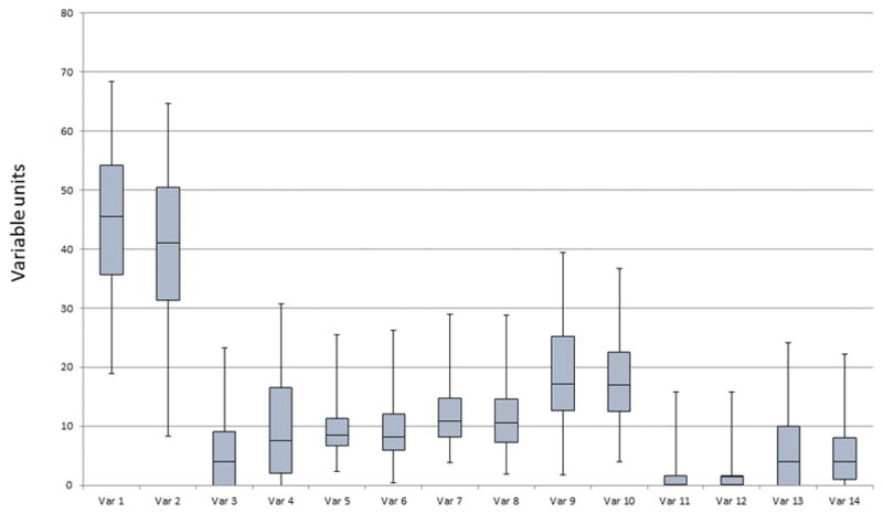
Example of a box plot.
The Shapiro-Wilks test [40] is useful to assess whether data are normally distributed, and the Kolmogorov-Smirnov test, although prone to low power, permits the investigator to compare the probability distribution of the sample data with that of a known probability distribution [41] or that of another sample set. The best guide is to observe the data and select an approach based on their distribution. Should the community of researchers expect an approach that is different than that suggested by the data, then, in addition to the procedure that the investigators believe the data requires, the investigators can take the approach suggested by the community and compare results from the two analyses.
When the investigators believe that reporting means and their measures of dispersion are appropriate, they should consider the choice of standard deviation versus the standard error. The standard error is simply the standard deviation of a sample mean, and it is smaller than the standard deviation. Which of these measures should be reported depends on the circumstances. If the investigators are interested in reporting the location and dispersion of individual observations in their sample set, then using the standard deviation permits the reader to assess the variability among observations. However, if the purpose is to show the value and variability not of the observations, but of the means, then the standard error should be used. However, once the investigators choose one of these measures of variability, they should be clear as to which they are providing.
Hypothesis testing tools
Hypothesis testing for dichotomous and polychotomous data
A list of statistical tests to assess common statistical hypotheses is available in Table 6. Investigators can test the null hypothesis for dichotomous data using Fisher’s exact test. In many cases, investigators will find that their data are polychotomous. Examples of these data include the Canadian Classification Score for Angina or the New York Association Heart Failure Score. In these cases, they can use Fisher’s exact test as well, since it is more accurate than chi-square testing, particularly when there is a small number of events in some variable categories.
Table 6.
Stat Methods
| Question to be Answered | Procedure | Advises on Application |
|---|---|---|
| One Sample Testing | ||
| Normality Assumption Valid | ||
| Is the population mean different than expected? | One sample t-test | Requires the sample size, mean, and standard deviation. |
| Distribution Free | ||
| Is the median of this distribution different than expected? | One sample Wilcoxon Signed Rank Sum Test | Requires the entire sample. |
| Two Sample Testing | ||
| Normality Assumption Valid | ||
| Do the means of two paired samples differ? | Paired t-test | Requires sample, mean difference and standard deviation of that difference. |
| Do the two independent samples have different means? | Unpaired t-test | Test variance first. Use equivariant solution for test on means if variances equal. Use unequal variance solution otherwise. |
| Distribution Free | ||
| Are the elements of two sequences mutually independent? | Spearman Rank Correlation Test | Requires entire data set; computes correlation based on ranks. |
| Are the data from paired samples from distributions with equal medians? | Wilcoxon Sign Rank Test | A paired difference test requiring all of the data. |
| Are the samples from the distributions with equal medians? | Wilcoxon Rank Sum Test (Mann-Whitney U Test) | Requires entire data set; computes a sum of signed ranks of the observations. |
|
More than Two Groups Normality Assumption Valid |
||
| Normality Assumption Valid | ||
| Do the predictor variables explain the response variable? | Regression analysis | Requires entire data set; adjusts for confounders; chunk testing is available; provides effect sizes and p-values. |
| Are there differences among the treatment group means? | Analysis of Variance | Requires entire data set; adjusts for confounders; blocking can be used; provides effect sizes and p-values. |
| Are their differences between different groups with multiple response variables? | Multivariate Analysis of Variance MANOVA | Requires entire data set; produces table related to analysis of variance table; effects for individual response variable must be analyzed separately. |
| Distribution Free | ||
| Are samples from each group from the same distribution? | Kruskal Wallis Test | Requires entire data set; provides results analogous to a one way analysis of variance. |
| Survival Analysis | ||
| Is there a difference in the time to event between the groups? | Kaplan Meier (log rank) | Requires for each subject the censoring category and time to event or end of follow-up; can manage more than two groups. |
| Can predictors explain the difference in time to event? | Cox proportional hazard analysis | Requires the entire data set; provides effect sizes as well as p-values. Adjusts for confounders |
Distribution-free hypothesis testing results—continuous data
Many distribution-free tests are available to investigators (Figure 2). When investigators examine their data and find that the distribution-free approach is best, they can conduct a one-sample assessment using the one-sample Wilcoxon sign rank test that determines the population median based on the sample. The investigators should anticipate the median value for the population under the null hypothesis. This test requires all of the data, not just the sample size, mean, and variance. Its output is the sample median and p-value.
Figure 2.

Flowchart of distribution free analysis for continuous data
Two-sample testing can be conducted using the two-sample Wilcoxon sign rank test if there is a natural pairing of the data. As with the one-sample test, all of the data are required, as the data are ordered and the ranks of each pair of data points are compared. The test addresses whether the medians of the two populations are different, and the output is the two medians and the p-value. The investigators can also conduct a two-sample Wilcoxon rank sum test (distribution-free) when the data consists of two unpaired samples. In this case, each of the observations from one sample is compared to the observations in the second sample, and a score is computed based on whether, within a data pair, the first group’s data point is greater than, equal to, or less than the second sample’s data point.
In some circumstances, the transformation of data that are not normally distributed to data that do follow the normal distributin can be quite useful. For example, in eventualities where the underlying data for a specific variable follow a log-normal distribution, this transformation is essential. In other cases, the mathematics underlying the variable’s development (e.g., those variables found in kinematics) provide a solid rationale for transformation. In these cases, the process the investigator can follow is to 1) transform the data, 2) carry out an analysis using parametric procedures, and then 3) apply the inverse transforms to convert the estimates of the mean and confidence intervals into the data with the original distribution.
Continuous data under a normal distribution
The investigators can avail themselves of several statistical tools when assessing the impact of an intervention on a continuous response variable that follows a normal distribution (Figure 3). When reporting data that is normally distributed, the investigators should report the effect size, the standard error (which is the standard deviation of the effect size), and the 95% confidence interval. The most useful statistical test for the investigator is the t-test. There are essentially three types of t-tests; 1) one-sample, 2) two-sample, paired, and 3) two-sample, unpaired. The latter can be conducted when either the variances of the two groups are considered equal or are believed to be unequal. In each case, all that is required is the sample size, mean, and standard deviation of the measures of interest from each group.
Figure 3.

Flowchart of regression analyses.
If investigators have response measures from n subjects and wish to test whether the population from which they selected their sample has a particular mean value, they would conduct a one-sample test based on the mean response variable value X̄ and the standard deviation sx. The output of this analysis is the mean, 95% confidence interval for the population mean, and p-value.
If investigators have an interest in tracking changes in a response variable over time, then each subject will have a measure at baseline Xb and a measure at follow-up Xf. In order to assess the change in response, the investigators can conduct a paired t-test, since each subject has a baseline and follow-up measurement, with the baseline measurement providing information about the follow-up measurement. This information provided by one measure about the other permits a smaller estimate of the variance, and therefore a more powerful hypothesis test. Here, the output is the sample means and standard deviations for each of the two groups, the 95% confidence interval for the difference in means, and the p-value.
If investigators have two groups of subjects that differ in a particular characteristic, and they are interested is testing whether the means of the two populations are different, then the two-sample t-test would serve the researchers well. As before, the output of the analysis is the sample means and standard deviations for each of the two groups, the 95% confidence interval for the difference in means, and the p-value. However the exact computation for the p-value depends on whether the variances in the two samples can be considered equal. Typically, statistical software provides the results for both the scenario where the investigators assume the variances are equal (and can therefore be pooled across the two groups) and also when the variances are assumed to be different. A separate hypothesis test can be conducted to assess the equality of variance assumption.
There is sometimes confusion about the best analysis to perform in a study where there is a control and a response group and each subject has a baseline and follow-up measurement. It is common for investigators to use two paired t-tests to determine if 1) the change in the response of the control group is statistically significant, and 2) the change in the response of the active group is statistically significant; however, this approach is suboptimal. A better approach to use is to compute for each group the mean change from baseline to follow-up and the standard error, and then to compare these mean changes using a two-sample unpaired t-test. However, investigators are well advised to avoid t-testing when the sample size of each group is extremely small (e.g., N = 3) and effect sizes are anticipated to be small or moderate. In this case, the researchers are better off with a one-sample sign test or two-sample Wilcoxon rank sum test. In addition, the investigators should keep in mind that one of the principal reasons to conduct hypothesis testing is to reliably determine whether results can be generalized from the sample to the larger population, a reliability that is undermined by the small size of the sample.
Analysis of variance (ANOVA)
Analysis of variance and regression modeling focus on building relationships between the response variable of interest and a collection of predictor variables (Figure 4). Investigators can use these procedures to assess whether the values of predictor variables change the response variable’s mean.
Figure 4.

Flowchart of parametric analyses for analysis of variance.
The fundamental concept behind ANOVA is that subjects treated differently will differ more than subjects treated the same. Even though it is the arithmetic means of the response variables that are examined across the predictor variables, the analysis is principally focused on converting “unexplained” variability to “explained” variability. If a variable is completely unexplained, then the investigator does not know why one subject’s measure is different than that of another. Identifying predictor variables provides an explanation for these differences, thereby reducing the unexplained variability. The inclusion of each new predictor variable increases the percent of the total variability that is explained, an increase that is reflected in an increased R2 [42].
Researchers can randomize subjects to one type of variable but with multiple levels (e.g., a single variable “diet” which comprises three different and distinct diets). They are interested in assessing whether there are any differences among these levels of the response variable. Because there are more than two groups in this type of analysis, a single t-test is inappropriate. While the investigators could conduct several different t-tests, the multiple testing issue must be addressed in order to avoid type I error inflation. Alternatively, an ANOVA test could be conducted to assess the degree to which the supplements explain differences in the rats’ left ventricular ejection fraction (LVEF) measurements. Since supplements are essentially the same class of predictor variable, the analysis is a one-way ANOVA. The F-statistic provides the overall test of significance.
Having conducted the ANOVA, investigators are commonly interested in assessing which group had the greatest effect on the response variable. This is the multiple testing problem, and the investigators are faced with comparing pairs of interventions (commonly referred to as contrasts),. Dunnett’s test is useful when the investigator is interested in testing several different interventions against a single control, and it is relatively easy to implement [43]. Scheffé’s method constructs confidence intervals simultaneously for multiple hypothesis tests and is helpful in ANOVA. [44] Tukey’s test permits the investigator to identify differences in means that have passed statistical testing, while correcting for multiple comparisons [45]. These are important tools available to the investigator that should be considered during the design of a research protocol.
A distribution-free analog to the one-way ANOVA that is available to investigators is the Kruskal-Wallis procedure. [46] It can be used to compare the distributions of two or more samples in a one-way ANOVA.
Factorial designs
The ANOVA model just described provides a structured set of procedures to determine if a set of more than two conditions has an effect on the response variable. However, research designs are increasingly complex, allowing deeper analyses of the relationship between a response variable and a predictor variable. In particular, factorial designs and blocking permit the investigator to examine the relationship between multiple predictor variables and the response variable, and at the same time decrease the response variable’s unknown variability. For this procedure, data on the response variable and each of the predictor variables must be available at the subject level.
A factorial design examines the impact of multiple dichotomous or polychotomous explainer variables on the response variable. In this case, the investigator is interested in each relationship. Consider an example where an investigator is interested in assessing the effects of two factors on LVEF recovery post infarction. In each pig, the researcher assesses the change in LVEF over time. One factor is the provision of granulocyte colony stimulating factor (G-CSF) one week prior to the beginning of the infarction. The second factor is the presence of mesenchymal stem cells (MSCs), which are delivered immediately post infarction. The investigators randomly choose whether the pigs receive G-CSF alone, MSC alone, both treatments, or a placebo. This two-by-two design permits an assessment of the overall effect of each of the G-CSF and MSC effects. It also evaluates whether the effect of MSC cells will be more pronounced in the presence of G-CSF than in its absence. This is traditionally known as an interaction, but is more helpfully described as an effect modifier, i.e., the effect of MSC is modified by the presence of G-CSF. The estimates of the main effects of G-CSF and MSC, as well as an effect modification, give this design a unique name: factorial design. Three and higher dimension factorial designs are also possible. From a variability reduction perspective, this is a very efficient design. The investigators can assess the influences of G-CSF and MSC, both separately or together, to reduce the unexplained variability in LVEF.
Blocking designs
Blocking designs, as with factorial designs, evaluate the relationship between multiple dichotomous or polychotomous explainer variables on the response variable. However, unlike the factorial design, where the researcher is interested in each relationship, in the blocking design, the researcher is only interested in the relationship between some of the predictor variables and the response variable. Variables that have a relationship with the response variables, but in which the investigator has little interest, are used to explain (or “block”) and eliminate variability in the response variable.
Using the previous example as a foundation, consider now the investigator who is interested in assessing the effects of G-CSF on the change in LVEF. Here, either G-CSF or the placebo is randomly provided to pigs immediately post infarction. However, the second factor for this experiment is not MSC, but is instead the size of the myocardial infarction.
The similarity of this design (G-CSF and myocardial infarction size as explainer variables) with the previous example (G-CSF and MSC as the explainer variables) is both helpful and misleading. Each design has two dichotomous explainer variables, and contains data in each of four cells. Therefore, mathematically, they can be analyzed the same way. However, there is a major difference. In the factorial design, each of the factors, G-CSF and MSC, were assigned randomly and the investigators were interested in the effects of each. In the second design, only G-CSF was randomly allocated. Infarct size could not be predetermined and assigned, and could very well be a surrogate for other variables, (e.g., condition of the LV before the myocardial infarction occurred or factor precipitating the myocardial infarction). In fact, the investigators are not particularly interested in assessing the effect of myocardial infarction on ΔLVEF.
However, this established relationship between infarct size and ΔLVEF is used to the investigator’s advantage. Since the infarct size-ΔLVEF relationship is well understood, the investigators know that myocardial infarct size will substantially reduce the unknown variability of ΔLVEF. This reduction in unknown variability is akin to reducing the surrounding noise, a procedure that will make it easier to detect the relationship of G-CSF to ΔLVEF. In this case, the infarct size is a “blocking variable,” i.e., it is of no real interest itself, but it reduces the background noise, making it easy to detect the G-CSF-ΔLVEF signal.
Repeated measures testing
The repeated measures design refers to research in which subjects have multiple measurements over time. These designs are useful when investigators are interested in assessing the effect of time on the distribution of observations. The simplest repeated measures analysis is a paired t-test, in which there are two measurements per subject. These designs can be expanded to many measurements over time (time is considered the “within subjects” variable, as well as to designs where there are measurements between subjects, e.g., control versus treatment (“between subjects”) variables. Cross-over designs are adaptations of repeated measure designs.
An efficiency introduced by the repeated measures design is the ability to directly assess the relationship between the response variables over time. While the researcher’s knowledge of the first subject’s baseline response measurement tells them nothing about the next subject’s measurement (the sine qua non of independence), knowing subject one’s baseline response can inform the investigator about that individual’s responses in the future. If these responses are linearly dependent (i.e., the fact that subject one’s baseline response is above the average baseline level makes it more likely that subject one’s response in the future will be above average) then a positive correlation is present. Just as in the ANOVA discussed above, the F-statistic determines the statistical significance of the time effect.
However, it is important for the investigators to recognize two critical assumptions in classical repeated measures design. The first is that this evaluation assumes an underlying normal distribution for the response variable. If the response variable is not normally distributed, or is not linear over time, then researchers can consider transformations of the data. In addition, investigators can carry out the Friedman test to assess differences over time when the response variables are ordinal, or when they are continuous but violate the normality assumption.
A second assumption in classical repeated measures designs is the compound symmetry assumption (i.e., there is equal correlation between the data points over all times). Modern computing programs permit the investigator to use the precise correlation structure in the dataset to be evaluated. In addition, the researcher can adjust the overall degrees of freedom used in the evaluations with the Greenhouse-Geisser, Huynh-Feldt, and lower bound procedures.
Multivariate analysis (MANOVA)
Investigators can turn to multivariate analyses when they are interested in assessing the effects of multiple predictor variables on the differences in means of multiple response variables. This procedure uses the correlation between multiple response variables to reduce the unexplained variability. Essentially, the multiple response variables are converted into one multidimensional response variable, and the statistical analysis assesses the effects of the predictor variables on this response variable vector.
For example, if the investigators are interested in assessing the effect of Ckit+ cells, MSC cells, and the combination of these two cell types on LVEF post myocardial infarction, they could assess these cell effects by ANOVA. However, deciding on a single response variable that determines LV function can be a challenge. Alternatively, they could measure LVEF, LVESVI, LVEDVI, and infarct size as response variables and conduct one MANOVA for these four variables.
The multivariate analysis generates an assessment of the effects of Ckit+ cells, MSC cells, and the combination of all four response variables. This analysis is a very efficient process, producing one p-value for all of these evaluations, and it is most useful when the result is null. If the investigators conducted an ANOVA on each of the four response variables, the multiplicity problem would be daunting (four hypothesis tests per ANOVA and four ANOVAs). However with MANOVA, should at least one relationship be statistically significant, the investigator must conduct a series of contrasts to determine where in the system the significant relationship lies. Also, like ANOVA, MANOVA hypothesis testing is based on the underlying normality of the individual response variables. When the observations do not follow a normal distribution, the investigator can transform the data to normality. If this is not possible, then permutation tests can be useful.
Regression analyses and adjusting for influences in normal data
Relationship building plays a pivotal role in understanding the true nature of the relationship between the response variable and the predictor variable. As pointed out earlier, ANOVA is useful when the response variable is continuous and the predictor variables are dichotomous or polychotomous in character. However, commonly, the predictor variables are continuous as well. In this case, the investigator can carry out regression analyses.
These analyses require the entire data set. When there is only one predictor variable, the regression analysis assesses the strength of the association between the response and the predictor variable, and the R2 value indicates the percent of the total variability of the response variable that is explained by the predictor variable. When more than one predictor variable is included in the regression model, the analysis indicates the strength of the association between the response and each of the predictor variables, adjusted for the effect of the other predictor variables. P-values are produced for each variable in the regression analysis.
As an example, suppose that a team of investigators is examining the change in LVEF over time in human subjects with heart failure and ongoing ischemia. These patients had their baseline CD34 phenotypes assessed. The investigators are interested in understanding the relationship between the response variable ΔLVEF and the predictor variable CD34. A simple regression analysis demonstrates the strength of the relationship between the two variables (Table 7). If the R2 from this model is 7.9%, then this indicates that 7.9% of the total variability of ΔLVEF is due to CD34, leaving most of the variability (100*[1−.079] = 92.1%) in this simple model to be is explained by factors other than the baseline CD34 phenotype.
Table 7.
Regression Analyses and Adjustment on δLVEF
| CD34 only model | |||||||
|---|---|---|---|---|---|---|---|
| Variable | DF | Parameter Estimate | Standard Error | t Value | Pr > |t| | ||
| Intercept | 1 | −3.28340 | 1.47829 | −2.22 | 0.0293 | ||
| CD34 | 1 | 1.28326 | 0.49991 | 2.57 | 0.0122 | R-Square | 0.0788 |
| Age only model
| |||||||
| Variable | DF | Parameter Estimate | Standard Error | t Value | Pr > |t| | ||
| Intercept | 1 | 8.53181 | 3.59827 | 2.37 | 0.0201 | ||
| Age | 1 | −0.12680 | 0.05608 | −2.26 | 0.0265 | R-Square | 0.0601 |
| CD34 and Age model
| |||||||
| Variable | DF | Parameter Estimate | Standard Error | t Value | Pr > |t| | ||
| Intercept | 1 | 3.18055 | 3.4.12730 | 0.77 | 0.4433 | ||
| Age | 1 | −0.09309 | 0.05559 | −1.67 | 0.0981 | ||
| CD34 | 1 | 1.08682 | 0.50789 | 2.14 | 0.0356 | R-Square | 0.1116 |
Using this same table, the investigators see that there is a quantitative relationship between ΔLVEF and CD34. It can be written as
They can reject the null hypothesis that there is no relationship between CD34 and ΔLVEF, and can explain the effect size from this model as follows: if there are two patients, and one has a CD34 level one unit higher than the other, then, on average, the ΔLVEF of the patient with the higher CD34 level will be 1.28 absolute LVEF units greater than the other. The p-value associated with this relationship is 0.012. Thus, the investigators would conclude that 1) there is a statistically significant relationship between ΔLVEF and CD34, and 2) the relationship still leaves most of the variability of ΔLVEF unexplained.
Now suppose that the investigator expected that ΔLVEF might also be explained by age and analyzes this new variable. The result of that analysis shows an R2 = 6.1%, coefficient = −0.127, and p = 0.027. From this analysis, the investigators have learned that just as there was a statistically significant relationship between ΔLVEF and CD34, there is also a statistically significant relationship between ΔLVEF and age. In the latter case, the relationship is
These results suggest that older subjects having a lower ΔLVEF level. However, identifying these two relationships begs the question: Of the two variables, CD34 and age, which is more closely related to ΔLVEF? This requires the research team to be familiar with the concept of statistical adjustment.
Adjustment
The notion of adjustment is different for researchers. To some, adjustment is synonymous with “control,” or in this circumstance, keeping age “constant” to assess the effect of baseline CD34 levels on ΔLVEF. This would be achieved by 1) choosing an age, and 2) carrying out a regression analysis relating ΔLVEF to CD34 for individuals only of that age. This is difficult to carry out, of course, because there are typically not enough individuals with the same age (or in an age “stratum”) that would permit a useful assessment of the ΔLVEF-CD34 relationship.
To biostatisticians, adjustment means something quite different then “control.” It means identifying, isolating, and then removing the influence of the adjusted variable on the relationship between the two other variables. This is the process of controlling for confounding, or understanding the way in which two predictor variables are co-related and therefore confound or conflate the relationship that each of them has with LVEF.
Regression analysis achieves this adjustment by 1) identifying and isolating the relationship between ΔLVEF and age, removing this effect from ΔLVEF, then 2) identifying the relationship between age and CD34 and removing this effect from CD34. 3) Evaluating the relationship between what is left of the CD34 effect on ΔLVEF completes the adjusted analysis. This process of isolating, identifying, and removing effects is precisely what multiple regression analysis achieves. Specifically, the result of this complex sequence of evaluations is the output of a regression analysis that relates ΔLVEF to both CD34 and age when they are both in the same model.
From the table, with both variables in the model, the total variability has increased to 11.2% which is greater than that of either CD34 by itself or age by itself. The overall model keeps the same directionality of the relationship, i.e., ΔLVEF is decreased by age and is larger in subjects with larger CD34 measures. However, the significance of the CD34 effect remains after the adjustment (i.e., after identifying, isolating, and removing the effect of age). Note, however, that the statistical significance of the ΔLVEF-age relationship is lost after adjusting for CD34. Thus, the age-adjusted CD34 relationship with ΔLVEF remains significant, while the CD34-adjusted age relationship with ΔLVEF does not.
Investigators should be aware of some cautions concerning regression analyses. With small datasets, the regression model is likely to be overspecified, providing so close a fit to the dataset that the results are of little value for the population at large. In this circumstance, partitioning the data into a dataset from which the model was created, and a second (and sometimes third) dataset on which the model is tested increases the validity of the model.
Statistical software is quite adept at building complex models that can explain a substantial proportion of the variability in dependent variable values. However, while a small number of predictor variables may have important impacts on the dependent variable, other predictor variables that are in the model, while also having a measurable impact on the dependent variable, are less influential. Therefore, when investigators face a model with a substantial number of predictor variables, they may be able to simplify the message conveyed to the research community by focusing on the two or three predictor variables that have the greatest impact.
An alternative approach to regression model building is to test an ensemble or group of effects for several predictor variables simultaneously. In this case, the investigators consider a model with and without this group of predictor variables. These “chunk tests” are straightforward, but require the investigators to know how to bundle subsets of predictor variables so that group-variable effects can be more easily interpreted.
Survival analysis and logistic regression
Survival analysis with Cox regression and logistic regression are regression procedures in which the response variable is a dichotomous variable or the combination of a response variable and a continuous variable (time to event).
Researchers can take advantage of the flexibility of dichotomous endpoints in the estimation of event rates. For example, if the investigators are interested in assessing the first occurrence of an event, e.g., the heart failure hospitalization rate over one year, then the proportion of such cases is the incidence rate discussed earlier.
Investigators use survival analyses when they want to examine and compare the survival of groups of individuals treated differently [47]. Survival is the time to an event (e.g., time to first hospitalization or time to death). The quantity of interest is the average time to event, and this is commonly compared between a control group and treatment group. It is a very straightforward process when the investigators know the survival time of each individual. However, this knowledge is frequently unavailable for all subjects. Kaplan-Meier life tables[48], log rank testing [49], and Cox regression analyses [50, 51] are most helpful to investigators in this case.
In analyses where subjects are followed for a proscribed period, investigator knowledge of the fate of each subject can be limited, and this limitation has an impact on the analysis. In a mortality study, for example, if a subject dies during the trial and the death date is known, then the investigators can use the survival time of that individual in their analysis; this subject is uncensored and the duration of survival is known. However, subjects may disappear from the study but not necessarily be dead. In these cases, the researcher only knows when the subject was last seen in the study, but does not know their current event status after they removed themselves from the research.* All that is known is that the individual survived up to the time of last contact. This survival is considered censored. These subjects are removed from follow-up after their last visits, and their removal is censored. Finally, subjects can reach the end of the study without an event occurring at all, denoted as administrative censoring. These different occurrences can all affect the estimates of mean survival times in the study.
Kaplan-Meier estimates rank the data by survival time in the study, and, then, using the censoring mechanisms, compute the number of subjects at risk of death in a time period, and, from that, determine the proportion of those at risk of death who actually die. This is assembled for the duration of the study to compute estimates of the overall survival rates. Cox hazard regression permits the investigator to conduct regression analyses on time to event/censored data. Here, there are two response variables: 1) whether the subject’s final status is censored or uncensored, and 2) the individual’s follow-up time in the study. Predictor variables were reviewed above. Cox regression produces as its output the relative risk associated with the predictor variable (through an exponentiation of the product of the coefficient and the predictor variable) and the p-value associated with that relative risk.
Alternatively, proportions can be used to estimate prevalence, e.g., the proportion of the population that has ever been hospitalized for heart failure. In retrospective studies, where the investigator starts with the number of cases and cannot differentiate incident cases from those that have been present in the population for a while, the investigator must rely on prevalence measures. If the investigators have only the prevalences for the control and intervention groups pc and pt, they can compute the prevalence . While this is related to the incidence ratio, it can be difficult for an intervention to have an impact on this ratio if the background rate (which is not affected by the intervention) is large.
In an assessment of prevalence, investigators can compute a more helpful quantity, the odds, which for the control group would be . This can take any value greater than zero, and with this value, it becomes easier to think of a regression model that would be based on it. In order to compare two groups, the odds ratio can be used. Odds ratios greater than one indicate that the treatment is more closely associated with the event than the control, and odds ratios less than one indicate that the odds of the event are lower for the treatment than for the control group.
Another advantage of odds ratios is that investigators can produce them from logistic regression analyses. [52] The response variable in a logistic regression is most commonly a dichotomous variable. The predictor variables can be either continuous or discrete. In addition, as was the case for regression analysis, logistic regression can accommodate multiple predictor variables. The exponentiated coefficient of a dichotomous predictor variable from a logistic regression analysis is an odds ratio. This procedure, therefore, permits the investigators to model the odds ratio as a function of covariates, and produces analysis tables that would be familiar to investigators who understand how to interpret this value from a regression analysis.
Combined endpoints
An adaptation available to investigators in clinical trials is a combined endpoint. In this case, the investigators combine multiple endpoints into one single but complex event. Researchers will face complications in the design of these endpoint structures, so the design must be based on an appropriate rationale.
There are advantages and disadvantages to this approach. When each component endpoint of the combined endpoint is dichotomous, the combined endpoint has a higher frequency of occurrence that will decrease the trial’s sample size. This can also decrease the cost of the trial. However, there are complications that come with the combined endpoint. If the combined endpoint has a nonfatal component, data collection can present a new administrative burden since it now requires an assessment to determineif the nonfatal component for any subject (e.g., hospitalization for heart failure) meets the study criterion.. This increases the cost and complexity of the study.
In addition, the use of combined endpoints can complicate the interpretation. The most straightforward conclusion to the study would be if all components of the combined endpoint are influenced in the same direction by the intervention. Any discordance in the findings of the component endpoints vitiates the impact of the intervention and undermines any argument that the treatment was effective.
However, even with these difficulties, combined endpoints have become an important adaptation in clinical trials. They are most useful if four principals are followed (Table 8), adapted from [53]. Both the combined endpoint and each of its component endpoints must be clinically relevant and prospectively specified in detail. Each component of the combined endpoint must be carefully chosen to add coherence to the combined endpoint, and should be measured with the same scrupulous attention to detail. The analysis of the therapy’s effect on the combined endpoint should be accompanied by a tabulation of the effects of the intervention on each component endpoint.
Table 8.
Principles of Combined Endpoints
| Principle of Prospective Deployment: Both the combined endpoint and each of its component endpoints must be clinically relevant and prospectively specified in detail. |
| Principle of Coherence: Each component of the combined endpoint must be carefully chosen to add coherence to the combined endpoint. |
| Principle of Precision: Each of the component endpoints must be measured with the same scrupulous attention to detail. |
| Principle of Full Disclosure: The analysis of the effect of therapy on the combined endpoint should be accompanied by a tabulation of the effect of the therapy for each of the component endpoints. |
In addition, investigators should avoid the temptation to alter the composite endpoint and its prospectively declared type I error structure during the course of the study. This tempting midcourse correction can lead to studies that are difficult to interpret [54,55,56]. In addition, changing components of the combined endpoint based on an interim result is often unsuccessful, since such interim findings are commonly driven by sampling error. Therefore, investigators should adhere closely to the prospective analysis plan.
Subgroup analyses
A subgroup analysis is an evaluation of a treatment effect in a fraction of the subjects in the overall study. These subjects share a particular characteristic (e.g., only males, or only patients with phenotype CD34 levels below a specific value). There are several justifiable reasons for investigators to conduct subgroups analyses. However, they should know that these analyses are also fraught with difficulty in interpretation. [57,58]
Commonly, the investigator simply and innocently wishes to determine whether the effect seen in the overall study applies to a specific demographic or comorbid group. This search for homogeneity of effect can be instigated by the investigators of the study. This evaluation can also be requested by journal reviewers and editors, or the entity that sponsors the research. Even the U.S. Food and Drug Administration (FDA) conducts subgroup analyses on data presented to it. Subgroup analyses are ubiquitous in the clinical trial literature, typified by Peto-grams† or forest plots that allow one to quickly scan down a figure and determine whether any of the subgroups are “off center,” i.e., well to the right or left of the main effect.
However, there are four main difficulties with subgroup analyses (Table 9). The first is that these analyses are not commonly considered before the beginning of a study, and fall into the rubric of exploratory analyses. Therefore, although they are provocative, they are rarely generalizable.
Table 9.
Problems with Subgroup Analyses
|
A second difficulty is that subgroup membership may not be known at baseline. Thus, not just the endpoint effect, but subgroup membership itself may be influenced by the intervention. Perhaps the most notorious example is the “as treated” analysis, frequently conducted during clinical trials, in which the treatment may have an influence (such as an adverse effect) that pushes patients assigned to the treatment group into those not receiving the treatment. Thus, the therapy appears to be more effective than it is, since only comparing those who could take the medicine and respond are compared with those who did not. Not even the prospective declaration of an “as treated” analysis can cure this problem. The third, lack of adequate power, and fourth, p-value multiplicity, are statistical, and undermine the generalizability of these within-subgroup effects.
Subgroups analyses have received substantial attention in clinical trial methodologies. However, investigators are best advised to treat provocative subgroup findings like “fool’s gold.” Caveat emptor.
Interim monitoring and other adaptive procedures
Up until this point in the review, the requirement for prospective planning in research has been emphasized. The intervention to be studied, the characteristics of the study population, the number of study arms, the number of endpoints, and the sample size of the study should all be identified prospectively. Then, once established, the protocol should be followed in detail. The advantage of this procedure is that the results of the study are more likely to be generalizable than with ad hoc analyses. However, even though this ability to apply the study’s results to the population at large is ideal, it is also inflexible. Might there not be some advantage to other approaches to research?
The need for protocol resilience is clearest when there is an ethical reason to end the study early because of early therapeutic triumph [59] or early catastrophe [60]. Since investigators carrying out the trial must remain blind to therapy assignment, a special oversight board with access to unblinded data (the Data Safety and Monitoring Board, or DSMB) is charged with reviewing the data well in advance of the completion of subject follow-up.
In so doing, these groups are required to consider action based on compelling but incomplete data. Several quantitative tools, called group sequential procedures (procedures that examine data from groups of subjects sequentially), were specifically designed to assist in these complex determinations [61]. Although the mathematics are somewhat complicated here, the concepts are quite simple.
First, if a study is to be ended prematurely, the data must be more persuasive than the minimal acceptable efficacy, had the trial been permitted to proceed to its conclusion. Second, the earlier the study is stopped, the more persuasive these findings must be. In addition, because data are examined repeatedly (although more data are added for each interim examination), there is a price one pays for multiple examinations of the data (and multiple p-values). Although this price is quite modest [62], an adjustment must be made.
However, perhaps the most important part of these interim examinations is non-statistical. Issues such as internal consistency (Do primary and secondary endpoint align?), external consistency (Have these results been seen in other studies?), biologic plausibility, and data coherence must also show that the interim data support a unified conclusion. All of these factors must be considered together for the decision to prematurely end a study.
Now, it is not uncommon for the DSMB to examine not just endpoint data for signs of early efficacy or early harm, but to examine the event rate in the placebo group of a clinical trial in order to recommend either increasing or decreasing the follow-up period based on the observed rate. If the endpoint is continuous, then its standard deviation can be appraised in real time. Each of these procedures is designed to test the assumptions of the underlying sample size computation, “adapting’ the computation to the actual data. Multi-armed clinical trials, e.g., studies designed to evaluate the effects of multiple doses of the agent in question, can have the sample sizes in specific arms increased or decreased, depending on the effect seen in that treatment arm. Each of these possibilities must be described in detail in the protocol, but once specified, they can be implemented without prejudice to the trial. The FDA has recently produced a draft guideline on adaptive clinical trial design [63]
The principal motivation for these rules is the conservation of resources. Subjects, workers, materials, and financial resources are rapidly consumed in research. In an era of increasing resource consciousness, careful planning for potential mid-course corrections that would save on trial cost and maintain ethical standards of the study is a laudable goal. However, the investigator must remember that 1) they are engaged in sample-based research, 2) the process of drawing generalizable conclusions from sample-based research is challenging, and 3) the smaller the sample size that a researcher is working with, the more likely one is to be misled.
Bayesian analyses
Bayesian approaches are becoming increasingly common in biostatistics, and in some circumstances, can represent a viable alternative to hypothesis testing. The investigator who uses a Bayesian analysis has an alternative to the classic p-value. Essentially, the investigator begins with a probability distribution of the parameter of interest. The data are then used to update this probability, essentially converting the prior probability distribution into a posterior probability. This permits the investigator to address specific questions of direct relevance, e.g., “What is the probability that the effect size of the study is greater than zero?” In addition, using a loss function permits the researchers to compute an estimate of the treatment effect known as the Bayes estimate. One must take care, however, in choosing the prior distribution and loss function. Adaptive designs (i.e., allowing interim evaluations of efficacy to determine the ratio of treatment to control group subjects to reduce the overall sample size of the study) are becoming more common.
Common mistakes to avoid
Most epidemiologic and biostatistics mistakes in cardiovascular research derive from one flaw—an inadequately prepared protocol. In its absence, the researcher is left to flounder in a rushing river of administrative, recruitment, and logistical issues that threaten to swamp any modern research effort.
Authors of a good protocol recognize at once the information needed to conduct the research effort successfully. The scientific question is essential. From this, endpoints are derived that define the instruments for measurement that will be used, followed by a determination of the number of treatment groups, and then a calculation of the required sample size and duration of the study. Dwelling on these concerns early simplifies the execution of the study.
When investigators have a solid, carefully considered, and well-written protocol, they are best advised to adhere to it. There will be many temptations to change. Other studies with interesting findings will be reported, leading investigators to new questions they may wish to pursue. New measurement tools will be discovered. Regulatory agencies may change direction. It is rare occurrence that these interceding events strengthen the study; instead, they threaten its vitiation. Investigators should maintain their commitment to the protocol in these circumstances. They can certainly report exploratory analyses, but these analyses must be acknowledged as such and not be permitted to overshadow the findings of the primary endpoints, whether they are positive or negative.
In addition, investigators should acknowledge and obtain any epidemiologic or biostatistical support that they need. The statistical analyst should keep the statistical analysis as simple as possible. The focus of the investigator’s query is to answer a cardiovascular question, and the study should be designed and the analysis conducted as simply as possible. The computations should be in line with the standards and expectations of the cardiology community. If a new computation is required, the investigators should precede this by using the standard computation, so that investigators can compare the two and come to a conclusion regarding the added value of the new approach. In this type of research, the statistics should be like the solid foundation of a house: all but invisible to the naked eye, but providing the solid basis from which to determine the exposure-disease relationship.
Investigators who are mindful of the methodologies depicted here can produce research results that permit the community to assimilate their conclusions. There is no doubt that there will be disappointments along the way, as data have no obligation to provide support for a researcher’s incorrect ideas. Data do, however, provide a window to the true state of nature, and through that, illumination.
Supplementary Material
Acknowledgments
The four reviewers’ suggestions and comments have been quite helpful.
Sources of Funding: Partial salary support for Dr. Moyé was provided by the National Heart Lung and Blood Institute under cooperative agreement UM1 HL087318.
Abbreviations
- LVEF
Left Ventricular Ejection Fraction
- MSC
Mesenchymal Stem Cells
- LV
Left Ventricular
- G-CSF
Granulocyte Stimulating Factor
- ANOVA
Analysis of Variance
- MANOVA
Multivariate Analysis
- CAD
Coronary Artery Disease
Footnotes
Some of the more eyebrow-raising reasons why subjects do not finish studies are that they are fleeing the law, have left their spouse for a surreptitious partner, are active traders in illegal narcotics businesses, are in prison, or are members of an organized crime network.
Named for the eminent British biostatistician, Richard Peto.
Disclosures: Dr. Moyé has no conflicts to report.
References
- 1.Schor S, Karten I. Statistical evaluation of medical journal manuscripts. JAMA. 1966;195:1123–8. [PubMed] [Google Scholar]
- 2.Hemminki E. Quality of reports of clinical trials submitted by the drug industry to the Finnish and Swedish control authorities. Eur J Clin Pharmacol. 1981;19:157–65. doi: 10.1007/BF00561942. [DOI] [PubMed] [Google Scholar]
- 3.George SL. Statistics in medical journals: a survey of current policies and proposals for editors. Med Pediatric Oncol. 1985;13:109–12. doi: 10.1002/mpo.2950130215. [DOI] [PubMed] [Google Scholar]
- 4.Ioannidis JPA. Why most published research findings are false. PLoS Med. 2005;2:e124. doi: 10.1371/journal.pmed.0020124. [DOI] [PMC free article] [PubMed] [Google Scholar]
- 5.Nuzzo R. Scientific method: statistical errors. Nature. 2014;506:150–2. doi: 10.1038/506150a. [DOI] [PubMed] [Google Scholar]
- 6.Kusuoka H1, Hoffman JI. Advice on statistical analysis for Circulation Research. Circ Res. 2002;91:662–71. doi: 10.1161/01.res.0000037427.73184.c1. [DOI] [PubMed] [Google Scholar]
- 7.Glantz SA. Biostatistics: how to detect, correct and prevent errors in the medical literature. Circulation. 1980;61:1–7. doi: 10.1161/01.cir.61.1.1. [DOI] [PubMed] [Google Scholar]
- 8.Lang T, Secic M. How to report statistics in medicine: annotated guidelines for authors, editors, and reviewers. Philadelphia, PA: American College of Physicians; 1997. [Google Scholar]
- 9.Landis SC, Amara SG, Asadullah K, et al. A call for transparent reporting to optimize the predictive value of preclinical research. Nature. 2012;490:187–91. doi: 10.1038/nature11556. [DOI] [PMC free article] [PubMed] [Google Scholar]
- 10.Multiple risk factor intervention trial. Risk factor changes and mortality results. Multiple Risk Factor Intervention Trial Research Group. JAMA. 1982;248:1465–77. [PubMed] [Google Scholar]
- 11.Feldman AM, Bristow MR, Parmley WW, et al. Effects of vesnarinone on morbidity and mortality in patients with heart failure. N Engl J Med. 1993;329:149–55. doi: 10.1056/NEJM199307153290301. [DOI] [PubMed] [Google Scholar]
- 12.Cohn J, Goldstein SC, Feenheed S, et al. A dose dependent increase in mortality seen with vesnarinone among patients with severe heart failure. N Eng J Med. 1998;339:1810–16. doi: 10.1056/NEJM199812173392503. [DOI] [PubMed] [Google Scholar]
- 13.Pitt B, Segal R, Martinez FA, et al. on behalf of the ELITE Study Investigators. Randomized trial of losartan versus captopril in patients over 65 with heart failure. Lancet. 1997;349:747–52. doi: 10.1016/s0140-6736(97)01187-2. [DOI] [PubMed] [Google Scholar]
- 14.Pitt B, Poole-Wilson PA, Segal R, et al. Effect of losartan compared with captopril on mortality in patients with symptomatic heart failure randomized trial–The losartan heart failure survival study, ELITE II. Lancet. 2000;355:1582–87. doi: 10.1016/s0140-6736(00)02213-3. [DOI] [PubMed] [Google Scholar]
- 15.Packer M, O’Connor CM, Ghali JK, et al. Effect of amlodipine on morbidity and mortality in severe chronic heart failure. N Engl J Med. 1996;335:1107–14. doi: 10.1056/NEJM199610103351504. [DOI] [PubMed] [Google Scholar]
- 16.Packer M. Presentation of the results of the Prospective Randomized Amlodipine Survival Evaluation-2 Trial (PRAISE-2) American College of Cardiology Scientific Sessions; Anaheim, CA: 2000. Mar 15, [Google Scholar]
- 17.Pfeffer M. Brigham and Women’s Hospital. Boston, Mass: Snell Medical Communications; 2000. A Second Prospective Randomized Amlodipine Survival Evaluation (PRAISE-2). Cardiology Scientific Update. [Google Scholar]
- 18.Packer M, Bristow MR, Cohn JN, et al. The effect of carvedilol on morbidity and mortality in patients with chronic heart failure. N Engl J Med. 1996;334:1349–55. doi: 10.1056/NEJM199605233342101. [DOI] [PubMed] [Google Scholar]
- 19.Moyé LA, Abernethy D. Carvedilol in Patients with Chronic Heart Failure (Letter) N Engl J Med; 1996;335:1318–1319. doi: 10.1056/NEJM199610243351711. [DOI] [PubMed] [Google Scholar]
- 20.Packer M, Cohn JN, Colucci WS. Response to Moyé and Abernethy. N Engl J Med. 1996;335:1318–1319. [Google Scholar]
- 21.Fisher L. Carvedilol and the FDA approval process: the FDA paradigm and reflections upon hypotheses testing. Cont Clin Trials. 1999;20:16–39. doi: 10.1016/s0197-2456(98)00054-3. [DOI] [PubMed] [Google Scholar]
- 22.Fisher LD, Moyé LA. Carvedilol and the Food and Drug Administration Approval Process: An Introduction. Controlled Clinical Trials. 1999;20:1–15. doi: 10.1016/s0197-2456(98)00052-x. [DOI] [PubMed] [Google Scholar]
- 23.Moyé LA. P Value Interpretation in Clinical Trials. The Case for Discipline. Cont Clin Trials. 1999;20:40–49. doi: 10.1016/s0197-2456(98)00051-8. [DOI] [PubMed] [Google Scholar]
- 24.Fisher LD. Carvedilol and the Food and Drug Administration-Approval Process: A Brief Response to Professor Moyé’s article. Cont Clin Trials. 1999;20:50–51. doi: 10.1016/s0197-2456(98)00052-x. [DOI] [PubMed] [Google Scholar]
- 25.Anonymous. Evidence of cause and effect relationship in major epidemiologic study disputed by judge. Epi Monitor. 1988;9:1. [Google Scholar]
- 26.Hill AB. The Environment and Disease: Association or Causation? Proceedings of the Royal Society of Medicine. 1965;58:295–300. doi: 10.1177/003591576505800503. [DOI] [PMC free article] [PubMed] [Google Scholar]
- 27.Miller RG. Simultaneous statistical inference. 2. New York: Springer-Verlag; 1981. [Google Scholar]
- 28.Zhang J, Qwuan H, Ng J, Stepanavage ME. Some statistical methods for mulitple endpoints in clinical trials. Cont Clin Trials. 1997;18:204–221. doi: 10.1016/s0197-2456(96)00129-8. [DOI] [PubMed] [Google Scholar]
- 29.Wright SP. Adjusted P-values for simultaneous inference. Biometrics. 1992;48:1005–1013. [Google Scholar]
- 30.Moyé LA. Multiple Analyses in Clinical Trials: Fundamentals for Investigators. New York, NY: Springer; 2003. [Google Scholar]
- 31.The CAST Investigators. Preliminary Report: effect of encainide and flecainide on mortalithy in a randomized trial of arrhythmia suppression after myocardial infarction. N Engl J Med. 1989;3212:406–412. doi: 10.1056/NEJM198908103210629. [DOI] [PubMed] [Google Scholar]
- 32.He Y. Missing data analysis using multiple imputation: getting to the heart of the matter. Circ Cardiovasc Qual Outcomes. 2010;3:98–105. doi: 10.1161/CIRCOUTCOMES.109.875658. [DOI] [PMC free article] [PubMed] [Google Scholar]
- 33.Rubin DB. Multiple Imputation for Nonresponse in Surveys. New York: Wiley; 1987. [Google Scholar]
- 34.Moyé LA, Davis BR, Hawkins CM. Analysis of a Clinical Trial Involving a Combined Mortality and Adherence Dependent Interval Censored Endpoint. Statistics in Medicine. 1992;11:1705–1717. doi: 10.1002/sim.4780111305. [DOI] [PubMed] [Google Scholar]
- 35.Moyé LA, Lai D, Jing K, Baraniuk MS, Kwak M, Penn MS, Wu CO. Combining censored and uncensored data in a U-statistic: design and sample size implications for cell therapy research. Int J Biostat. 2011;7:Article 29. doi: 10.2202/1557-4679.1286. [DOI] [PMC free article] [PubMed] [Google Scholar]
- 36.Rosner B. Fundamentals of biostatistics. Boston, Mass: Brooks/ Cole; 2011. [Google Scholar]
- 37.When to Use a NonParametric Testhttp://sphweb.bumc.bu.edu/otlt/MPH-Modules/BS/BS704_Nonparametric/BS704_Nonparametric2.html
- 38.Krzywinski M, Altman N. Points of Significance: Visualizing samples with box plots. Nat Methods. 2014;11:119–120. doi: 10.1038/nmeth.2813. [DOI] [PubMed] [Google Scholar]
- 39.Streit M, Gehlenborg N. Points of View: Bar charts and box plots. Nat Methods. 2014;11:117–117. doi: 10.1038/nmeth.2807. [DOI] [PubMed] [Google Scholar]
- 40.Shapiro SS, Wilk MB. An analysis of variance test for normality (complete samples) Biometrika. 1965;52:591–611. [Google Scholar]
- 41.Pearson ES, Hartley HO, editors. Biometrika Tables for Statisticians 2. Cambridge University Press; 1965. pp. 117–123. Tables 54, 55. [Google Scholar]
- 42.Kutner M, Nachtsheim C. Applied Linear Statistical Models. 5. New York, NY: McGraw Hill; 2004. [Google Scholar]
- 43.Dunnett CW. New tables for multiple comparisons with a control. Biometrics. 1964;20:482–491. [Google Scholar]
- 44.Scheffé H. The Analysis of Variance. New York: Wiley; 1999. [Google Scholar]
- 45.Montgomery DC. Design and Analysis of Experiments. 8. Hoboken, NJ: Wiley; 2013. Section 3.5.7. [Google Scholar]
- 46.Corder GW, Foreman DI. Nonparametric Statistics for Non-Statisticians. Hoboken: John Wiley & Sons; 2009. pp. 99–105. [Google Scholar]
- 47.Cook TD, DeMets DL. Statistical Methods for Clinical Trials. 1. Boca Raton, FL: Chapman Hall; 2008. [Google Scholar]
- 48.Kalbfleisch JD, Prentice RL. The statistical analysis of failure time data. New York: John Wiley; 1980. [Google Scholar]
- 49.Mantel N. Evaluation of survival data and two new rank order statistics arising in its consideration. Cancer Chemotherapy Reports. 1966;50:163–70. [PubMed] [Google Scholar]
- 50.Breslow NE. Analysis of Survival Data under the Proportional Hazards Model. International Statistical Review / Revue Internationale de Statistique. 1975;43:45–57. [Google Scholar]
- 51.Cox DR. Regression Models and Life-Tables. Journal of the Royal Statistical Society. 1972;34:187–220. [Google Scholar]
- 52.Hosmer DW, Lemeshow S, Sturdivant RX. Applied Logistic Regression. 3. Hoboken, NJ: Wiley and Sons; 2013. [Google Scholar]
- 53.Moyé LA. Multiple Analyses in Clinical Trials: Fundamentals for Investigators. New York: Springer; 1993. [Google Scholar]
- 54.UK Prospective Diabetes Study Group. UK Prospective Diabetes Study (UKPDS) VIII - Study, design, progress and performance. Diabetologia. 1991;34:877–890. [PubMed] [Google Scholar]
- 55.Turner RC, Holman RR on behalf of the UK Prospective Diabetes Study Group. The UK Prospective Diabetes Study. Finnish Medical Society DUOCECIM. Ann Med. 1998;28:439–444. doi: 10.3109/07853899608999105. [DOI] [PubMed] [Google Scholar]
- 56.UKPDS Study Group. Intensive blood glucose control with sulphonylureas or insulin compared with conventional treatment and risk of complications in patients with type 2 diabetes. Lancet. 1998;352:837–853. [PubMed] [Google Scholar]
- 57.Assmann S, Pocock S, Enos L, Kasten L. Subgroup analysis and other (mis)uses) of baseline data in clinical trials. Lancet. 2000;355:1064–69. doi: 10.1016/S0140-6736(00)02039-0. [DOI] [PubMed] [Google Scholar]
- 58.Yusuf S, Wittes J, Probstfield J, Tyroler HA. Analysis and interpretation of treatment effects in subgroups of patients in randomized clinical trials. JAMA. 1991;266:93–8. [PubMed] [Google Scholar]
- 59.DeMets DL, Hardy R, Friedman LM, Lan KK. Statistical aspects of early termination in the beta-blocker heart attack trial. Control Clin Trials. 1984;5:362–72. doi: 10.1016/s0197-2456(84)80015-x. [DOI] [PubMed] [Google Scholar]
- 60.The CAST Investigators. Preliminary Report: effect of encainide and flecainide on mortalithy in a randomized trial of arrhythmia suppression after myocardial infarction. N Engl J Med. 1989;3212:406–412. doi: 10.1056/NEJM198908103210629. [DOI] [PubMed] [Google Scholar]
- 61.Reboussin DM, DeMets DL, Kim KM, Lan KK. Computations for group sequential boundaries using the Lan-DeMets spending function method. Control Clin Trials. 2000;21:190–207. doi: 10.1016/s0197-2456(00)00057-x. [DOI] [PubMed] [Google Scholar]
- 62.Lan KK, Wittes J. The B-value: a tool for monitoring data. Biometrics. 1988;44:579–85. [PubMed] [Google Scholar]
- 63.Draft guidance for industry and food and drug administrative staff. Adaptive designs for medical device clinical studies. Draft Guidance. http://www.fda.gov/ucm/groups/fdagov-public/@fdagov-meddev-gen/documents/document/ucm446729.pdf.
Associated Data
This section collects any data citations, data availability statements, or supplementary materials included in this article.