

A high-throughput biological small-angle X-ray scattering facility is described, which combines single-channel robotic pipetting with a capillary-based sample cell. The design parameters, sample rinsing protocol and effects of fluid dynamics on radiation damage are examined.
Keywords: biological small-angle X-ray scattering, robotics, microfluidics
Abstract
With the rise in popularity of biological small-angle X-ray scattering (BioSAXS) measurements, synchrotron beamlines are confronted with an ever-increasing number of samples from a wide range of solution conditions. To meet these demands, an increasing number of beamlines worldwide have begun to provide automated liquid-handling systems for sample loading. This article presents an automated sample-loading system for BioSAXS beamlines, which combines single-channel disposable-tip pipetting with a vacuum-enclosed temperature-controlled capillary flow cell. The design incorporates an easily changeable capillary to reduce the incidence of X-ray window fouling and cross contamination. Both the robot-control and the data-processing systems are written in Python. The data-processing code, RAW, has been enhanced with several new features to form a user-friendly BioSAXS pipeline for the robot. The flow cell also supports efficient manual loading and sample recovery. An effective rinse protocol for the sample cell is developed and tested. Fluid dynamics within the sample capillary reveals a vortex ring pattern of circulation that redistributes radiation-damaged material. Radiation damage is most severe in the boundary layer near the capillary surface. At typical flow speeds, capillaries below 2 mm in diameter are beginning to enter the Stokes (creeping flow) regime in which mixing due to oscillation is limited. Analysis within this regime shows that single-pass exposure and multiple-pass exposure of a sample plug are functionally the same with regard to exposed volume when plug motion reversal is slow. The robot was tested on three different beamlines at the Cornell High-Energy Synchrotron Source, with a variety of detectors and beam characteristics, and it has been used successfully in several published studies as well as in two introductory short courses on basic BioSAXS methods.
1. Introduction
While small-angle X-ray scattering has enjoyed a long and productive history in materials and polymer science (Guinier, 1969 ▶), its popularity in biology is a relatively recent phenomenon made possible by a confluence of algorithmic advances, the availability of synchrotron sources and the changing needs of researchers in molecular biology (Nagar & Kuriyan, 2005 ▶). Continuing advances in computation have pushed biological small-angle X-ray scattering (BioSAXS) far beyond the basic structural parameters and model testing once associated with the method. As such, it now plays an important complementary role in molecular and structural biology (Jacques & Trewhella, 2010 ▶). The inherently low resolution and heavily averaged nature of biological small-angle solution scattering is offset to a considerable degree by its versatility. Data can be collected from a wide range of solution conditions without the need for crystals. In addition to projects such as structural genomics, which naturally generate large numbers of samples, routine BioSAXS itself requires multiple dilutions of every sample to control for interparticle interference and possible concentration effects. Furthermore, variations in buffer composition, pH, ionic strength and additives are often of interest. Unlike protein crystallography, which presents a unique challenge in mounting and centering cryogenically cooled solid samples, solution scattering experiments can utilize well established liquid-handling technology. This makes BioSAXS a natural candidate for automation.
Automated BioSAXS sample-loading systems of various designs have appeared at several beamlines worldwide. EMBL beamline X33 at DESY (Hamburg, Germany) first introduced a system capable of handling up to 192 samples in the 80–100 µl volume range. Using a needle, the robotic system extracted sample volumes from microcentrifuge tubes with pierceable lids and delivered them to the flat-walled sample cell via a length of polytetrafluoroethylene tubing (Round et al., 2008 ▶). Beamline ID14-3 at ESRF (Grenoble, France), in collaboration with EMBL, has recently commissioned a new sample changer based on this design that reduces the sample loading and cleaning cycle down to 30 s (Pernot et al., 2010 ▶). The new design minimizes the flow path by moving the sample plates rather than the needle. Like the system we present here, it also utilizes a thin-walled 2 mm quartz capillary in vacuo as a sample cell. Quartz capillaries are perhaps the most widely used sample cell type at present (Lipfert et al., 2006 ▶; Dubuisson et al., 1997 ▶).
The SIBYLS beamline at the Advanced Light Source (Berkeley, USA) has adapted a commercial liquid-handling robot (Hamilton Robotics Inc., Reno, NV, USA) to fill static flat-windowed sample cells. By focusing a highly convergent X-ray beam on the detector, the dose is spread throughout the sample volume (12 µl), reducing potential radiation damage (Hura et al., 2009 ▶). BioSAXS Beamline 4–2 at SSRL (Stanford, USA) uses a small-footprint custom sample changer, but with a cannula that inserts directly into a capillary flow cell. This unique design allows the cannula to seal directly to the capillary entrance so that a single syringe pump doubles for both sample delivery and sample flow within the X-ray cell (Weiss, 2011 ▶).
Microfabricated fluid flow systems have been used in the study of time-dependent phenomena, such as unfolding and photoinduced conformational change (Pollack & Doniach, 2009 ▶; Lamb et al., 2008 ▶). Microfluidic lab-on-a-chip systems capable of mixing multiple components have also been introduced (Toft et al., 2008 ▶; Nielsen, 2009 ▶; Lafleur et al., 2011 ▶). Separation technology has proven vital to good-quality BioSAXS data. Both Soleil (Paris, France) and APS (Argonne, USA) have coupled high-performance liquid chromatography systems to beamlines to improve sample purity and to facilitate data capture on structurally unstable biomolecules (David & Pérez, 2009 ▶; Mathew et al., 2004 ▶).
The automated high-throughput sample-changing system described here is a hybrid approach, incorporating disposable-tip automated pipetting and a capillary flow cell. The small-footprint commercial pipetting robot loads an in vacuo capillary flow cell from up to three standard 96-well trays. To reduce sample cross-contamination and X-ray window fouling, this design combines disposable-tip pipetting with rapidly changeable quartz capillary sample cells. A unique vortex chiller design is used to keep sample plates cool, and sample evaporation is minimized with commercial pre-pierced adhesive film. The Python-based robot-control and data-processing software packages described here form an integrated BioSAXS structure pipeline that is easily operated by novice users. In addition to design considerations, we also examine sample consumption, the cleaning protocol and how the fluid dynamics within capillary cells redistribute X-ray-damaged material. Test results from three different Cornell High-Energy Synchrotron Source (CHESS) beamlines with various beam and detector characteristics are presented. The system has been successfully used in published structural studies and as a teaching tool in two introductory BioSAXS workshops.
2. Experimental
2.1. Beamlines
The robotic sample changer and cell described here are portable. To evaluate performance in a variety of environments with different beam characteristics, we have tested the system on three different beamlines at CHESS. Table 1 ▶ gives beamline characteristics and typical experimental parameters. F2 station, originally designed for multi-wavelength anomalous diffraction, is equipped with an Si(111) monochromator with horizontal saggital focusing. While it produces the sharpest energy resolution of the three beamlines, its beam profile is broader and more non-uniform in the horizontal direction than the other two lines. The horizontal capillary arrangement used in this study is particularly advantageous in this case since it can accommodate horizontally broad beams without spillover. Both G1 and G3 stations utilize W/B4C multilayers. The broader energy distribution (ΔE/E = 0.015 for G1 and ΔE/E = 0.02 for G3) results in significantly higher flux densities and correspondingly shorter sample exposure times. For practical reasons G3 station was operated at the lowest energy of the three. Because the sample path length of 2 mm in our cell design is optimal for 10 keV radiation, absorption for lower energies will be higher. For water in this energy range, absorption has approximately cubic wavelength dependence (Stuhrmann, 1978 ▶). If the transmitted intensity relative to the incident beam is  with a path length of
  and
and  (cm−1), we can choose
  cm at wavelength λF2 = 1.24 Å for optimum signal in our apparatus at F2 station. The relative attenuation factor for a sample at λG3 = 1.45 Å would then be
  , incident intensities being equal. The signal reduction at this lower wavelength is therefore modest assuming comparable detector efficiency.
Table 1. Beamline characteristics and experimental parameters.
| Station | F2 | G1 | G3 |
|---|---|---|---|
| Energy (keV) | 9.881 | 9.869 | 8.580 |
| Beam size (µm) | 250 × 250 | 250 × 250 | 250 × 250 |
| Flux (photons s−1) | 9 × 10⁹ | 3 × 10¹¹ | 1 × 10¹¹ |
| Sample–detector distance (mm) | 1130 | 1190 | 1540 |
| Typical exposure time (s) | 30–180 | 3–15 | 5–30 |
At all three stations, the direct beam was placed at the bottom center of the detector surface to maximize q-space range. [Throughout this work, we define q = 4πsin(θ)/λ, where 2θ is the scattering angle and λ is the wavelength.] While this configuration (a 50° wedge for ADSC Q1 and FLICAM, 23° wedge for Pilatus 100K-S detectors) does not capture the full circle of scattered photons for a given q value, it does minimize horizontal beam smearing. The degree to which wider integration ranges contribute to improved signal depends upon the uniformity of detector response across the face, a quantity that could vary by as much as 1% (Krumrey & Ulm, 2001 ▶; Gruner et al., 2002 ▶; Owen et al., 2009 ▶).
The same optical table and components were used for both F2 and G3. Tungsten slit blades were polished and tested for parasitic scatter on a laboratory source in vacuo (Advanced Design Consulting USA Inc., Lansing, NY, USA). The first set of slits was used to define the beam, while the second set was used to remove parasitic scatter. Beam flight paths start with a 25 µm-thick mica vacuum window just upstream of the first pair of defining slits (Attwater Group, Preston, Lancashire, UK). The path is kept under vacuum (2–10 mtorr ≃ 0.27–1.33 Pa) to minimize air scatter. In F2 and G3, the beam-defining slits were separated from the guard slits by 365 mm; the guard slits were 200 mm from the sample. The distance necessary for freely moving vacuum bellows presently limits the guard slit distance to the sample. Transmitted beam intensity through the sample is monitored using an Si photodiode embedded in a tungsten cup and the integrated values are used to normalize buffer subtractions.
2.2. Sample preparation
Bovine serum albumin (BSA; 66 kDa; Sigma–Aldrich Corporation, St Louis, MO, USA) was prepared in 50 mM HEPES buffer pH 7.3. Glucose isomerase (173 kDa; Hampton Research, Aliso Viejo, CA, USA) was dialized into 100 mM Tris buffer, 1 mM MgCl2 pH 8. Ribonuclease A (13.7 kDa; gel-filtration calibration kit 17-0442-01, GE Healthcare, Piscataway, NJ, USA) was prepared in 100 mM Tris buffer, 100 mM NaCl pH 7.5. The lysozyme buffer contained 40 mM NaOAc (pH 4.0), 50 mM NaCl and 1% glycerol. All samples were centrifuged for 10 min at 14 000 r min−1 before exposure. Concentrations were measured using 280 nm UV absorption (NanoVue, GE Healthcare, Piscataway, NJ, USA).
3. Overall design
The automated sample-loading system consists of three principal components: a small-footprint pipetting robot capable of loading samples from three 96-well trays, a water-cooled sample flow cell with a 2 mm-diameter 10 µm-thick quartz capillary, and a fluid-handling system composed of a computer-controlled syringe pump and a liquid waste trap (Fig. 1 ▶).
Figure 1.

Schematic diagram of the automatic sample-loading system using standard hydraulic symbols. The robot pipettes the sample into the funnel and the sample is then drawn into the capillary sample chamber using the two-way syringe pump. After exposure, the sample passes into the waste trap vial.
3.1. Pipetting robot
A commercial pipetting robot, the Hudson SOLO high-throughput single-channel pipettor (Hudson Robotics Inc., Springfield, NJ, USA) (Fig. 2 ▶), was chosen on account of its small (14 × 16 inch ≃ 35.6 × 40.6 cm) footprint and unique overhang construction. The robot has four standard 96-well tray positions and is configured with a single OEM 100 µl Hamilton syringe pump. The included SOLOSoft control software, which provides a full array of calibration and liquid-handling functions via the RS232 protocol, is used primarily for station setup. Owing to the complexity of our overall system, custom Python-based open-source software was developed in-house to coordinate robot operation, sample cell flow and synchrotron beamline functions (§3.3). Pipette tips are automatically loaded and shucked as needed. The ability to use clean tips when loading new samples reduces cleaning time and minimizes potential contamination between samples. Sample trays are covered with a pre-cut film (X-Pierce Sealing Film, EXCEL Scientific Inc., Victorville, CA, USA) to prevent evaporation and can be kept cool with an airstream generated by a commercial vortex chiller (AiRTX International, Cincinnati, OH, USA). While the cooling temperature is not dynamically controlled, it is monitored by thermocouple and has been found to be sufficiently stable (< ±2 K) over time to prevent accidental sample freezing.
Figure 2.

Automated loading system as installed on the CHESS F2 beamline: (1) Hudson SOLO robot, (2) funnel to capillary, (3) sample cell camera, (4) angled mirror and (5) in-hutch sample cell monitor.
3.2. Sample flow cell
The sample cell design combines easily exchangeable capillaries with a short sample flow path. The sample-loading robot uses disposable pipette tips to deliver droplets to a specially designed funnel system where they are aspirated into the path of the X-ray beam by a syringe pump with a micro-solenoid valve (Aurora BioMed, Vancouver, BC, Canada). Easily interchangeable aluminium cartridges containing thin-walled quartz glass capillaries (Hampton Research, Aliso Viejo, CA, USA) with access holes for X-ray and visible light are sealed to the vacuum flight path using O-rings. One end of the rod can accommodate a flangeless chromatography fitting while the other is pressed into a standard O-ring face seal embedded in the funnel (Fig. 3 ▶). The capillary is sealed into the rod using standard epoxy cement. A borosilicate glass window allows users to view and position the sample plug in the X-ray beam via a 45° mirror and telescopic optics. The temperature in the aluminium block containing the capillary cartridge can be regulated using a standard water-circulating bath. The housing for the aluminium block contains vacuum-compatible KF40 bulkhead clamps (not shown) for easy integration into the beamline flight paths. Similarly to the SAXS cell design of Dubuisson et al. (1997 ▶), flexible bellows on either side of the housing allow the entire assembly to be freely aligned while under vacuum using a motorized x–z stage.
Figure 3.

Sample cell enclosure with changeable capillary. Quartz capillaries are embedded in reusable aluminium rods sealed to the enclosure by means of piston-style O-rings (1). A funnel connected to the capillary by face-seal O-rings allows sample plugs as small as 5 µl to be loaded either manually or by pipetting robot (2). The sample is visible from above through a borosilicate window (3). KF40 bulkhead clamps connect the entire assembly to beampipe bellows to facilitate x–z alignment (not shown). The inner aluminium block is temperature regulated via a standard chilled-water connection (4).
For typical beamline energies of 10 keV, a sample path of approximately 2 mm provides the maximum signal, subject to sample absorption, according to the classic 1/μ rule, where μ is the X-ray attenuation coefficient for water (Glatter, 1982 ▶) (see also §2.1 of the present paper). In a perfect BioSAXS environment where no parasitic background scatter is present, shorter path lengths should, in principle, reduce sample consumption by reducing the loss of scattered signal due to absorption. However, the inherently weak nature of SAXS signals and the reality of incomplete elimination of background scatter argue for the classic length. The design we present here, of course, can accommodate any capillary diameter.
For the purposes of calibration, the chromatography fitting at the end of the capillary cartridge can be removed and a soft small-diameter plastic capillary containing silver behenate (The Gem Dougout, State College, PA, USA) can be inserted to provide a d-spacing standard. Alignment of the sample cell is accomplished by scanning the filled cell while monitoring counts on the beamstop PIN diode. Routinely, a 700 µm-diameter scintillating terbium-doped glass fiber (Collimated Holes, Campbell, CA, USA) is inserted directly into the capillary as an extra visual check of X-ray beam alignment.
3.3. Fluid-handling system and software control
The entire sample-loading system is controlled by in-house software developed in the Python programming language. The control software, Robocon, provides a graphical user interface (GUI; Fig. 4 ▶) for controlling both the robot and the syringe pump, either individually or together using predefined functions. Robocon handles all communications with the robot and the bi-directional syringe pump via high-level serial commands. The software runs on a dedicated netbook controllable from anywhere on the network using a TightVNC (http://www.tightvnc.com) server, which enables it to be controlled by any device with an internet browser.
Figure 4.

Graphical user interface for Robocon control software. The sample can be adjusted dynamically during oscillation using the up/down arrows in the center panel. Stroke volume and pump speed are also dynamically adjustable. The volume of sample to be withdrawn from the 96-well tray is specified in the spreadsheet in the lower left. The interface also controls detector operation.
Information on the state of the robot and the pump is displayed in the GUI in the form of both a status message and an indicator light on the right of the GUI. A digital clock shows the remaining exposure time. The 96-well plate is displayed as a grid table where the desired aspirated sample volume can be entered and a label can be assigned to each well. The software is also able to control the beamline data acquisition software (SPEC/ADX) using the SpecClient Python library (http://forge.ill.fr/projects/specclient) and adjust all exposure parameters.
Sample positioning buttons enable control of the position of the sample plug in the capillary and oscillation/continuous flow operations. A series of automated sample loading, exposure and cleaning commands can be programmed using the Autorun feature by selecting wells and adding them to a loading-sequence list. All sample-loading operations are monitored on LCD screens using four miniature NTSC video cameras.
3.4. Data processing
The free open-source data-reduction software RAW (Nielsen, 2009 ▶) is an integral part of the system, providing easy data reduction, manipulation and analysis. RAW has been extended with numerous features to make it more portable between different beamlines. Supported detectors now include the Pilatus, Mar345 image plate, MAR165 CCD and ADSC images, as well as standard 16 and 32 bit TIFF formats. Normalization of profiles for buffer subtraction often requires reading and manipulation of the information found in the image header and/or accompanying counter files. RAW automatically reads the image header of a loaded image, and currently supports file header formats at beamlines at CHESS and MAXLab. Header data values can be combined in user-defined mathematical expressions before being used for normalization. Several new features have been added to improve workflow in the robotic environment, such as writing all analysis information to a comma-separated file that can be opened in a regular spreadsheet program, and the ability to quickly browse data and header information on plotted files. A new and improved indirect Fourier transform feature is currently under development. RAW is available at http://sourceforge.net/projects/bioxtasraw/ and currently runs on Windows, Linux and Mac platforms.
4. Performance
4.1. Sample-loading procedures
The typical procedure for loading a sample is as follows: using a fresh tip, the Hudson SOLO loads the sample from a 96-well tray and dispenses it in the funnel. A syringe pump (Aurora Biomed, Vancouver, BC, Canada) aspirates the sample from the funnel into the capillary and positions it in the path of the X-rays. The sample can be statically positioned, continuously flowed, or oscillated back and fourth in the X-ray path. A set of 11 consecutive 15 µl lysozyme buffer samples were loaded by the robot with no user intervention and evaluated for volume, position and X-ray profile consistency. Each sample was exposed on the CHESS F2 station for 30 s using a Pilatus 100 K-S detector (Dectris, Baden, Switzerland), integrated and normalized for transmitted intensity. The actual delivered volume as measured by plug length varied by 7.6% (1 µl) on average. The accuracy of the position of the plug relative to the beam varied by 9.5% of the total length. The variation between X-ray profiles as measured by  [for buffer sample k, let σk be the standard deviation of the profile I
k; each profile is sampled at N discrete q values between the limits q
min and q
max] yields an average χ2 = 1.05 with a standard deviation of 0.08. Fig. 5 ▶ shows every third sample profile (I
0, I
3, I
6, I
9) superimposed on the average profile and shifted horizontally for clarity. While the intensities increase slightly as the curve approaches the tail of the direct beam at low q and the edge of the detector at high q, consecutive buffer curves agree to within the shot noise of the experiment with no detectable drift.
[for buffer sample k, let σk be the standard deviation of the profile I
k; each profile is sampled at N discrete q values between the limits q
min and q
max] yields an average χ2 = 1.05 with a standard deviation of 0.08. Fig. 5 ▶ shows every third sample profile (I
0, I
3, I
6, I
9) superimposed on the average profile and shifted horizontally for clarity. While the intensities increase slightly as the curve approaches the tail of the direct beam at low q and the edge of the detector at high q, consecutive buffer curves agree to within the shot noise of the experiment with no detectable drift.
Figure 5.

Reproducibility of scattering profiles for consecutively loaded 15 µl lysozyme buffer samples. Solid lines represent the average of 11 consecutive profiles, while open circles represent individual samples. For clarity, only every third profile (I 0, I 3, I 6, I 9) is shown and displaced horizontally. From load cycle to load cycle, buffer profiles are stable to within the detector/shot noise level of the experiment.
Sample oscillation is widely used in BioSAXS as a means of reducing the effects of radiation damage, and it is the recommended data-collection mode at MacCHESS since it allows users to collect up to the radiation damage limit and then merge only undamaged images. After exposure, the sample is pulled through the capillary into a waste vial. Excess air volume in the present design can give rise to thermal drift of the sample plug during lengthy exposures on weaker beamlines. The Robocon software allows users to manually shift the plug position when necessary without interrupting sample oscillation. This issue is most pronounced after handling the waste vial, and can affect sample-loading and oscillation reproducibility until temperature equilibrium has been reached. To achieve better stability, future designs will incorporate less air volume within the fluid flow pipeline.
Sample loading and positioning is automated using in-house Python software with an intuitive GUI (Fig. 4 ▶). All data are automatically azimuthally averaged, normalized by incident intensity, and plotted using the RAW program (Nielsen, 2009 ▶). Protein standards are routinely taken at the beginning of every user run. Fig. 6 ▶ shows the scattering data and envelope for the relatively small protein ribonuclease A (13.7 kDa), obtained by oscillating a 20 µl plug of solution (10 mg ml−1). The computed scattering profile for the crystal structure [Protein Data Bank (PDB; Berman et al., 2002 ▶) code 1fs3; Chatani et al., 2002 ▶] is also shown for comparison. The radii of gyration (R g) as calculated by AutoRg (Petoukhov et al., 2007 ▶) suggest mild concentration effects [R g = 14.8 (4) Å at 10 mg ml−1, R g = 15.5 (2) Å at 5 mg ml−1] in comparison to the published value of 15.8 (4) Å (Mylonas & Svergun, 2007 ▶). The values obtained via the inverse Fourier method for both concentrations (R g = 15.26 and R g = 15.31, respectively) are more consistent and also in good agreement. For the purpose of this shape reconstruction, we opted to use the 10 mg ml−1 profile for a good signal quality at the widest angles.
Figure 6.

Computed versus experimental scattering data for ribonuclease A and glucose isomerase. SAXS envelopes, superimposed on known crystal structures, are obtained from the above scattering curves.
Results for the larger, but more dilute, glucose isomerase sample (173 kDa at 1 mg ml−1; PDB code 1oad; Ramagopal et al., 2003 ▶) are also shown in Fig. 6 ▶. From the Guinier analysis, R g = 32.8 (8) Å is in good agreement with the published value of 32.5 (7) Å. Glucose isomerase has been suggested as a particularly stable standard for BioSAXS (Kozak, 2005 ▶). Both data sets were collected with an exposure time of 180 s at the F2 beamline at CHESS.
Profiles of dilute bovine serum albumin solution collected on all three stations (F2, G1 and G3) are shown in Fig. 7 ▶. The expected scattering profile from the human homolog of serum albumin (PDB code 1n5u; Wardell et al., 2002 ▶) as computed with CRYSOL (Svergun et al., 1995 ▶) is given for comparison (currently no crystal structure for BSA is known). The data curves for F2 and G1 have been down-sampled by a factor of 2 (averaging pairs) to facilitate visual comparison. Similarly, profile G3 has been down-sampled by a factor of 4. The experiments on F2 and G3 shared the same 5 mg ml−1 BSA sample separated by six days. The BSA sample for G1 was more concentrated (7.8 mg ml−1). Exposure times of 180 s (F2), 20 s (G1) and 3 × 5 s (G3) yield doses of approximately 2 × 10¹², 6 × 10¹² and 2 × 10¹² photons, respectively. All curves have similar signal-to-noise characteristics, with the G1 sample giving the best signal of the three and F2 the weakest. The inset Guinier plot shows excellent agreement between F2 and G3 data, but slight concentration effects for the G1 sample, as might be expected. The measured R g values are 29.4 Å for F2, 29.3 Å for G1 and 29.9 Å for G3, in agreement with the published value 29.9 (8) Å (Mylonas & Svergun, 2007 ▶). It is important to note here that BSA has a known tendency towards aggregation and must be prepared fresh; consequently, glucose isomerase has been suggested as a better standard for BioSAXS (Kozak, 2005 ▶).
Figure 7.

Intensity profiles from dilute BSA solution measured on three different CHESS beamlines: F2, G1 and G3. The solid black line is the scattering profile for the closest known structure to BSA, human serum albumin. Exposure times have been chosen so that all three curves have approximately the same signal levels. The inset shows a Guinier plot in the region qR g < 1.3. The G1 data show a slight concentration effect.
4.2. Timing
The system is able to load and position a sample in 14 s. Introducing a tip change adds an additional 8 s. After loading, the sample plug can be oscillated to reduce radiation damage. Manual adjustments are currently needed to ensure the sample plug is positioned correctly for oscillation so that the full length of the sample plug is utilized to minimize radiation damage. These manual adjustments typically take of the order of 30 s. The time needed to load and make a sample ready for exposure with oscillation is thus close to 1 min in total. Capillary rinsing times are typically between around 1 min corresponding to loading and flushing three plugs of cleansing liquid, typically buffer. Detector readout times vary from 15–10 s on older CCD detectors to milliseconds or less on state-of-the-art direct detection systems. Currently, serial communication latency and backlash corrections limit the pump response to 250 ms. The total time for exposure of a sample and its corresponding buffer is 2–3 min depending on the cleaning procedure, which enables the system to run through 20–30 subtracted profiles per hour with exposure times of around 5 s.
4.3. Cleaning
Because of flow cell reuse, cleaning is a critical task. We have found that flushing 100–200 µl of buffer through the capillary between measurements in plugs of 50–70 µl is sufficient for most samples. Residue will eventually build up on the capillary walls, which needs more thorough cleaning. Fouling of the capillary seems to be the primary cause of flow disruptions through the capillary. We hypothesize that hydrophobic deposits on the otherwise hydrophilic glass surface can lead to uneven forces on the sample plug meniscus as it moves. In more serious cases, flow resistance can even lead to the sample plug diverting around the area of the beam position or to splitting of the plug, which causes bubble formation. This phenomenon dominates sample flow behavior in both horizontal and vertical capillary configurations. Following the practice suggested by David & Pérez (2009 ▶), we have found that mild detergent washes can restore even flow. It is unclear if this is a result of true cleaning or simply of detergent coating hydrophobic patches. Since the presence of detergent contamination, and other cleaning agents, is known to adversely affect SAXS measurements of proteins, rinsing after the application of detergent is essential. It is also important to flush with water prior to flushing with detergent to avoid possible deposition of denatured protein. For routine washes to resolve flow problems we employ a 2%(m/v) solution of the low-density zwitterionic detergent N-dodecyl-N,N-(dimethylammonio)butyrate (Hura, 2011 ▶). If a capillary cannot be changed between user groups, or if flow problems persist during a run, we have found that a 30 min soak in the more aggressive cleaning agent Hellmanex II (2% v/v) (Hellma Analytics, Müllheim, Germany) is effective at improving flow.
To test for completeness of rinsing, we compared a series of five BSA (7.8 mg ml−1) and buffer measurements, each separated by a cleaning with three plugs of 70 µl buffer. The buffer scattering profiles superimpose to within an average χ2 = 0.63 (9). Fig. 8 ▶(a) shows the intensity curve for the buffer with the largest deviation (χ2 = 0.77) superimposed on the initial buffer along with the corresponding BSA profile for reference. A plot of ΔI/σ for the residual intensity (the difference between the initial buffer and buffers taken after cleaning, all five samples superimposed) shows a barely perceptible upward trend at low angles, with few points above I/σ = 2.0 (Fig. 8 ▶ b). Residual protein signal is therefore not statistically significant after the three-plug 70 µl cleaning protocol.
Figure 8.

Effectiveness of sample cell rinse protocol. A series of five trial plugs of 7.8 mg ml−1 BSA solution were introduced into the sample cell, each separated by a cleaning of three plugs of 70 µl each of buffer followed by a final plug of buffer for comparison. The intensity profiles for the initial buffer (blue) and the buffer with the largest deviation from initial (trial No. 4 with χ2 = 0.77) (red) are shown superimposed in (a). For scale, BSA solution trial No. 4 is also shown in green. A plot of ΔI/σ for the residual protein intensity in the buffer for all five trials shows a barely perceptible upward trend at low angle, with few points above ΔI/σ = 2.0 (b). Residual protein signal is therefore not statistically significant after the cleaning protocol.
4.4. Sample consumption, radiation damage and flow within the capillary
The volume delivered by the robot was calibrated by weighting a pipette tip before and after loading with water. The accuracy of the measurement is approximately ±1 µl. The experiment was repeated to find the lowest possible volume that would reproducibly form a uniform movable plug in the capillary. The Hudson sample robot was able to reproducibly deliver sample volumes between 8 and 90 µl. Sample sizes smaller than 10 µl are difficult to reliably keep in the beam during oscillation because of thermal drift, so 12–20 µl is the recommended range for routine data collection by robot. The minimum of 10 µl is also the lower limit of working volume for the V-shaped-bottom 96-well trays, as recommended by the manufacturer (Nunc V96 MicroWell Plates, Nalge Nunc International, Rochester, NY, USA). Sample sizes as small as 5 µl can be loaded into the funnel manually. Such a small sample size approaches the practical limit of the system since it creates the smallest plug that can be sustained within the 2 mm-diameter capillary. Precisely how small a plug one can achieve depends upon the degree of hydrophilicity of the glass walls and the surface tension of the sample. Hydrophilic capillary surfaces are not only desirable for their fluid-handling properties but also thought to reduce protein binding and surface fouling (Castner & Ratner, 2002 ▶).
The beam diameter is generally chosen as a balance between the practically achievable minimum q (which varies linearly with beam diameter) and flux (Chu et al., 1994 ▶). Optimal beam diameters tend to be significantly smaller than sample path lengths. In our case, the 250 µm-diameter beam exposes only (0.25 mm)2 × 2.0 mm = 0.125 µl of sample out of the full cross-sectional volume of the capillary: 2π mm2 × 0.25 mm = 1.57 µl. So while the beam hits a relatively small flat region of the glass, only about 8% of the sample is exposed to the hottest part of the beam.
Thin-walled quartz capillaries, which are commonly used in BioSAXS, also introduce X-ray absorption of the order of 20% at 10 keV by our measurements. Future flat-walled cell designs offer the possibility of using more X-ray transparent window material. Fabricated sample cells with flat walls also offer the possibility of more efficient sample utilization, but cell dimensions still need to exceed the beam diameter by a wide margin to avoid accidental reflection of the tails of the beam profile off the side walls of the cell. For a Gaussian profile exp[−x
2/(2c
2)] with FWHM = 0.25 mm, c = 0.25/2 . For the profile of the direct beam to fall in intensity to levels comparable to that of the brightest scattering intensity of the sample [I(q = 0)/I
incident ≃ 10−6] (Stuhrmann, 1980 ▶), the effective beam width becomes
. For the profile of the direct beam to fall in intensity to levels comparable to that of the brightest scattering intensity of the sample [I(q = 0)/I
incident ≃ 10−6] (Stuhrmann, 1980 ▶), the effective beam width becomes  = 1 mm. This limitation makes an accurate assessment of radiation damage in BioSAXS difficult since the hot part of the beam cannot illuminate the full contents of the sample cell without creating parasitic reflections. Placing a guard aperture very close to the incoming cell window could reduce such reflections by more nearly replicating a square beam profile. Future cell designs will need to address this issue.
The advantage of using a flow cell is that fresh sample can be delivered to the X-ray beam while damaged material is flushed away. With unlimited sample volume, rapid constant flow can, in principle, reduce radiation damage to negligible limits. In situations with limited sample volume, oscillation of small liquid plugs allows users to collect multiple images up to and beyond the damage limit, then decide how many frames to merge into the final data set. The oscillation approach is also well suited to samples with unknown damage susceptibility.
If an oscillated sample is to be kept entirely within the quartz capillary, the upper limit for the sample volume is approximately 120 µl, though the stroke volume of the pump limits the oscillated volume to less than 100 µl. Larger sample volumes allow longer exposures to be taken without damage in the case of more dilute solutions where the signal is weak.
However, the question of whether to oscillate or flow sample is not as simple as it might appear. Fluid flow within a sufficiently small diameter capillary tube is not a simple case of translation. For a 2 mm-diameter capillary containing pure water at 277 K, the Reynolds number ( , where R = radius, U = plug velocity, ρ = density and μ = viscosity) falls below 1.0 when the flow rate falls below 2.4 µl s−1. At 6 s to span 15 µl of sample, this is a realistic, if slightly slow, flow rate for the higher-intensity beamlines at CHESS. This places sample transport well within the laminar flow regime but borderline with regard to the Stokes (creeping flow) approximation (Re << 1). Inertial and time-dependent pumping effects, which are neglected in the Stokes flow, are likely to be visible at the turning points of oscillation. Nonetheless, the Stokes equations become increasingly valid with smaller capillary sizes, more viscous protein solutions and slower flow rates. It is therefore informative to examine the Stokes flow solutions.
In the fluid mechanics literature, the behavior of a moving plug of liquid in a pipe is referred to as bolus flow. We utilize a three-dimensional analytical solution of the Stokes stream function to generate the velocity field and subsequent flow lines (Duda & Vrentas, 1971 ▶). Air–water boundaries are assumed to be flat and the velocity is zero at the capillary walls (the no-slip condition) (Appendix A ). As the plug is forced down the capillary by air pressure, friction against the walls pushes the outer sheath of fluid toward the rear of the plug. Having nowhere else to go, the liquid reverses direction and forms a forward-moving column up the center of the plug. The result is a vortex ring (Fig. 9 ▶ a). The effect can be seen experimentally by injecting a small volume of tracer dye into a 10 µl plug of water within our capillary cell (Fig. 9 ▶ b). The flat air–water boundary assumption is quite good on the leading surface of the plug as can be seen in the figure, but drag produces a curved boundary at the rear. Even for a uniformly moving plug, there is significant circulation of material. This phenomenon has long been known to enhance heat and gas transfer in fluids (Duda & Vrentas, 1971 ▶). Bolus flow can therefore serve as an effective mixing mechanism on the microfluidic scale.
Figure 9.

Fluid flow pattern within a 9.4 µl plug of water moving from right to left in a 2 mm-diameter capillary under air pressure. The simulated velocity field in the creeping flow limit (small Reynold’s number) shows a characteristic vortex ring pattern (yellow arrows) with toroidal-shaped isosurfaces of the stream function (levels of blue) in (a). The same flow pattern is made visible in an actual moving sample plug when tracer dye is added (b).
To understand how damaged material in the sample volume is mixed under continuous and oscillatory plug motion, we can integrate the flow field to generate streamlines (Appendix A ). To avoid unwanted reflections and parasitic scatter, a safety margin must always be observed to keep the X-ray beam away from the gas–liquid boundaries. The calculation uses a 3 mm liquid plug (9.4 µl) with the X-ray beam traversing the middle 2 mm. Since this model is axisymmetric, we plot only the cylindrical coordinates ±ρ and z. Fig. 10 ▶ shows the wake of damaged material left as the sample makes one oscillation period through the beam. Each plot represents the plug at the specified time. The position of the beam (vertical line) has been aligned in all three plots. The arrows indicate the direction of future movement and contours of the stream function are shown as dotted lines.
Figure 10.

Simulated wake of X-ray-damaged material as a sample plug oscillates in the X-ray beam. Each plot represents the plug at a different time, with the arrows indicating the direction of future motion. The vertical line (aligned in all three plots) is where the X-ray beam traverses the sample. Dotted lines are contours of the stream function. The damaged region swept out by the beam is shaded gray and undamaged regions are labeled A and B. The line thickness represents degree of exposure.
For creeping flow, reversal of plug motion is equivalent to time reversal of the internal circulation. In general, time-dependent pumping effects (change in plug velocity with time, such as at the turning points of oscillatory motion) will affect internal circulation whenever the change in velocity exceeds viscous effects in the fluid. For this basic analysis, we neglect those effects and assume a sluggish pump relative to the Re value.
The wake produced by the first pass through the beam passes back through the beam again to produce a doubly dosed wake of identical shape on the opposite side. As a result of volume conservation, the exposed volume of sample is exactly the same as would be obtained by moving the beam and holding the capillary fixed. There is an important difference in exposure, however: circulation in the vortex ring is not fast enough to bring previously damaged material back into the beam. While the velocity in the center is twice that of the plug motion (in the laboratory reference frame), the velocity of the boundary layer near the capillary surface is nearly zero. The slow moving boundary layer is thus heavily dosed before it can escape (wake lines converge at the glass in Fig. 10 ▶). This results in accumulation of damaged material near the wall of the capillary.
Unexposed sample volumes (regions A and B in Fig. 10 ▶) are alternately forced between the ends of the plug and the walls. Though these volumes never mix with damaged material in the creeping flow regime, they will have enhanced diffusive mixing due to their increased contact area with the damaged zone. This behavior is directly analogous to Taylor dispersion for sample injection in chromatography (Deen, 1998 ▶).
For a 2 mm-diameter capillary containing water, however, inertial and time-dependent pumping effects must be present to some extent. Sudden reversal caused by fast oscillation has been observed to produce complex flow patterns at the end of the plug that may contribute to mixing (not shown). More sophisticated computational fluid dynamics simulations would be necessary to determine if any significant azimuthal mixing occurs by this effect that would bring fresh material into the beam (Fujioka & Grotberg, 2004 ▶). Such effects, however, will diminish with capillary size.
It may be that adopting hydrophobic window material will relax the no-slip conditions that give rise to increased damage in the boundary layer, but research in microfluidic surface fouling tends to focus on hydrophilic surfaces (Castner & Ratner, 2002 ▶). The only way to completely mitigate the accumulation of damaged material in the boundary layer may be to adopt a moving-window strategy such as that advocated by Hong & Hao (2009 ▶).
5. Conclusions
An automated sample-loading robot with flow cell and integrated software for BioSAXS is presented. The design combines disposable-tip pipetting with a horizontal vacuum-enclosed capillary flow cell. Sample volumes between 90 and 10 µl can be handled by the robot with a throughput of approximately 20–30 profile measurements per hour including manual intervention. The sample may be manually loaded and recovered from the cell down to 5 µl. While the present flow cell runs in a supervised mode, full automation with no user intervention is planned by minimizing the air volume around the sample plug and installing a UV cell for both sample positioning and concentration measurements. While the sample cell design allows for easy change of capillaries, we have demonstrated that a minimal cleaning protocol, rinsing the capillary with three 70 µl plugs of buffer, is sufficient to reduce residual protein signal to below the limits of detection.
The portable robotic system has been tested on three different synchrotron beamlines at CHESS. Comparable results were obtained when exposure times were selected to compensate for differing beamline flux. Common protein standards reproduced the scattering profiles, radii of gyration and envelopes derived from published coordinates.
Flow within the capillary exhibits a unique vortex-ring pattern that circulates material between the walls and center of the tube as the plug moves. Because fluid flow in capillaries below 2 mm in diameter is close to the creeping flow limit, little actual mixing is expected. Quantitatively, moving a plug past a stationary beam exposes the same total volume of fluid that would be exposed if the beam were moving along a stationary plug, but the nature of damage accumulation is quite different. Because of the slow-moving fluid boundary layers with no-slip conditions, damaged material accumulates near the capillary surface. Vortex flow is not sufficient to bring previously damaged material back into the beam, and plug reversal that is sufficiently slow during oscillation does not expose new material in the creeping flow limit. The primary advantage of oscillation in the microfluidic regime is only that it allows users make more efficient use of a sample by taking multiple exposures and merging only non-damaged profiles.
The robotically loaded capillary flow system described here is routinely available to MacCHESS users on the F2 and G1 beamlines. The dramatically increased throughput of the system has made it possible to host training workshops in which a significant number of students can collect data on their own samples over the course of only two days (including lecture time). During the spring of 2011, MacCHESS offered two two-day training workshops on BioSAXS in which a total of 43 students attended, bringing 23 different sets of samples for collection on the two beamlines. Reduced effects of radiation damage due to flow have also proven advantageous to users. A number of studies have now appeared in the literature utilizing this system (Byrnes & Sondermann, 2011 ▶; Yennawar et al., 2011 ▶; Jiang et al., 2011 ▶).
Acknowledgments
Thanks to Mike Cook for producing the drawing of our sample cell (Fig. 3 ▶) and for designing and fabricating the vacuum components and supports for our optical table. Thanks also to Marian Szebenyi for adapting the MacCHESS data-collection software to communicate with the Robocon software and for implementing software for reading and correcting detector images and recording beam stop diode readings. Scott Smith, Bill Miller, Jennifer Kenkel and the CHESS engineering team were responsible for constructing the optical table used in both F2 and G3. Jon Kopsa machined critical O-ring components. James Savino designed the 96-well plate chiller used in this paper. Thanks to Arthur Woll for making the G1 and G3 stations available, and to Phil Sorensen for critical help with configuring station software and networking. Valuable discussions with James Holton on detectors were much appreciated. This research was conducted at CHESS, which is supported by the National Science Foundation and the National Institutes of Health/National Institute of General Medical Sciences under NSF award DMR-0225180, using the MacCHESS facility, which is supported by award RR-01646 from the National Institutes of Health, through its National Center for Research Resources.
Appendix A. Stokes’s equation for bolus flow
We present here a detailed discussion of the formula for bolus flow as it relates to sample-damage calculations in this paper. The full Stokes equation for fluid flow is traditionally written in dimensionless coordinates so that it may be simplified under conditions of steady flow, high viscosity and small size scales (Deen, 1998 ▶). In cylindrical coordinates, let z be the capillary axis, r the radial distance of a point from the axis and θ the angle about the axis. Further, let ( ) be scaled in such a way that
  and
and  , where β = capillary length/capillary radius. Writing the velocity
  , the Navier–Stokes equation becomes
where P is dynamic pressure. The key parameter, which sets the relative scale between inertial and viscous effects in fluid flow, is the Reynold’s number  . R is the tube radius, U is maximum velocity, ρ is density and μ is viscosity. In §4.4 we saw that Re falls near unity for the flow cell described here; consequently the left-hand side of equation (1) becomes less important as capillary diameters fall below 2 mm. Before we continue on that assumption, it is important to consider the Strouhal number
  (Deen, 1998 ▶). The time scale τ represents the period over which significant velocity changes can occur. In our case, this number is set by the speed with which the sample plug reverses direction during oscillation. For an ideal square wave, this value could be quite small, causing Re/Sr ≃ 1 even when Re << 1. For this study we neglect the term by assuming pump reversal is slow compared to viscous effects.
When expressed in cylindrical coordinates, flow through a capillary is axisymmetric and can be reduced to a problem of two dimensions (r, z). In the plug’s moving coordinate system, the capillary walls move backwards  while the air–water boundary remains stationary
  . Fluid is confined to within the capillary walls and cannot flow through the capillary axis:
  . The air–water interfaces (z = 0, β) and the capillary axis (r = 0) are no-drag boundaries leading to the derivative conditions
The method of stream functions elegantly reduces the system of second-order partial differential equations (the Navier–Stokes equation together with the continuity equation  ) to a single fourth-order equation. By defining
the continuity equation is automatically satisfied, and pressure can be made to drop out of the equation in the customary way (Duda & Vrentas, 1971 ▶). The result is the well known biharmonic equation
The boundary conditions for the stream function become  = 1 for moving capillary walls,
  = 0 for the stationary air–water interfaces and
 for confinement.
No-drag conditions for air–water interfaces and capillary axis must be expressed as derivatives:
Expressing the solution as a Fourier series,
the biharmonic equation yields a fourth-order ordinary differential equation that can be solved in terms of modified Bessel functions of the first kind (I 0, I 1 and I 2) (Duda & Vrentas, 1971 ▶):
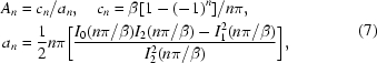 |
Expressions for the velocity field follow directly from equation (3):
by using the derivative relation
The explicit formula for the derivative term is thus
To obtain particle trajectories, the coupled system of ordinary differential equations
is solved numerically from specified initial conditions (r 0, z 0) using the Python SciPy algorithm odeint, which is derived from ODEPACK (Hindmarsh, 1983 ▶). In treating radiation-damaged zones by propagating lines of initial conditions in the flow, we have neglected the effect of diffusion, which is expected to be minor in the creeping flow limit.
References
- Berman, H. M., Westbrook, J., Feng, Z., Gilliland, G., Bhat, T. N., Weissig, H., Shindyalov, I. N. & Bourne, P. E. (2000). Nucleic Acids Res. 28, 235–242. [DOI] [PMC free article] [PubMed]
- Byrnes, L. J. & Sondermann, H. (2011). Proc. Natl Acad. Sci. USA, 108, 2216–2221. [DOI] [PMC free article] [PubMed]
- Castner, D. G. & Ratner, B. D. (2002). Surf. Sci. 500, 28–60.
- Chatani, E., Hayashi, R., Moriyama, H. & Ueki, T. (2002). Protein Sci. 11, 72–81. [DOI] [PMC free article] [PubMed]
- Chu, B., Harney, P. J., Li, Y., Linliu, K., Yeh, F. & Hsiao, B. S. (1994). Rev. Sci. Instrum. 65, 597–602.
- David, G. & Pérez, J. (2009). J. Appl. Cryst. 42, 892–900.
- Deen, W. M. (1998). Analysis of Transport Phenomena. New York: Oxford University Press.
- Dubuisson, J.-M., Decamps, T. & Vachette, P. (1997). J. Appl. Cryst. 30, 49–54.
- Duda, J. L. & Vrentas, J. S. (1971). J. Fluid Mech. 45, 247–260.
- Fujioka, H. & Grotberg, J. B. (2004). J. Biomech. Eng. 126, 567–577. [DOI] [PubMed]
- Glatter, O. & Kratky, O. (1982). Small-Angle X-ray Scattering. London: Academic Press.
- Gruner, S. M., Tate, M. W. & Eikenberry, E. F. (2002). Rev. Sci. Instrum. 73, 2815–2842.
- Guinier, A. (1969). Phys. Today, 22, 25–30.
- Hindmarsh, A. C. (1983). IMACS Transactions on Scientific Computation, Vol. 1, Scientific Computing, edited by R. S. Stepleman, pp. 55–65. Amsterdam: North-Holland.
- Hong, X. G. & Hao, Q. (2009). Rev. Sci. Instrum. 80, 1–8. [DOI] [PMC free article] [PubMed]
- Hura, G. L. (2011). Personal communication.
- Hura, G. L., Menon, A. L., Hammel, M., Rambo, R. P., Poole, F. L., Tsutakawa, S. E., Jenney, F. E., Classen, S., Frankel, K. A., Hopkins, R. C., Yang, S. J., Scott, J. W., Dillard, B. D., Adams, M. W. W. & Tainer, J. A. (2009). Nat. Methods, 6, 606–613. [DOI] [PMC free article] [PubMed]
- Jacques, D. A. & Trewhella, J. (2010). Protein Sci. 19, 642–657. [DOI] [PMC free article] [PubMed]
- Jiang, F., Ramanathan, A., Miller, M. T., Tang, G.-Q., Gale, M., Patel, S. S. & Marcotrigiano, J. (2011). Nature (London), 479 423–427. [DOI] [PMC free article] [PubMed]
- Kozak, M. (2005). J. Appl. Cryst. 38, 555–558.
- Krumrey, M. & Ulm, G. (2001). Nucl. Instrum. Methods Phys. Res. Sect. A, 467, 1175–1178.
- Lafleur, J. P., Snakenborg, D., Nielsen, S. S., Møller, M., Toft, K. N., Menzel, A., Jacobsen, J. K., Vestergaard, B., Arleth, L. & Kutter, J. P. (2011). J. Appl. Cryst. 44, 1090–1099.
- Lamb, J. S., Zoltowski, B. D., Pabit, S. A., Crane, B. R. & Pollack, L. (2008). J. Am. Chem. Soc. 130, 12226–12227. [DOI] [PMC free article] [PubMed]
- Lipfert, J., Millett, I. S., Seifert, S. & Doniach, S. (2006). Rev. Sci. Instrum. 77, 1–3.
- Mathew, E., Mirza, A. & Menhart, N. (2004). J. Synchrotron Rad. 11, 314–318. [DOI] [PubMed]
- Mylonas, E. & Svergun, D. I. (2007). J. Appl. Cryst. 40, s245–s249.
- Nagar, B. & Kuriyan, J. (2005). Structure, 13, 169–170. [DOI] [PubMed]
- Nielsen, S. S. (2009). PhD thesis, Technical University of Denmark, Kongens Lyngby, Denmark.
- Owen, R. L., Holton, J. M., Schulze-Briese, C. & Garman, E. F. (2009). J. Synchrotron Rad. 16, 143–151. [DOI] [PMC free article] [PubMed]
- Pernot, P., Theveneau, P., Giraud, T., Nogueira Fernandes, R., Nurizzo, D., Spruce, D., Surr, J., McSweeney, S., Round, A., Felisaz, F., Foedinger, L., Gobbo, A., Huet, J., Villard, C. & Ciprianai, F. (2010). J. Phys. Conf. Ser. 247, 012009.
- Petoukhov, M. V., Konarev, P. V., Kikhney, A. G. & Svergun, D. I. (2007). J. Appl. Cryst. 40, s223–s228.
- Pollack, L. & Doniach, S. (2009). Methods Enzymol. 469, 253–268. [DOI] [PubMed]
- Ramagopal, U. A., Dauter, M. & Dauter, Z. (2003). Acta Cryst. D59, 868–875. [DOI] [PubMed]
- Round, A. R., Franke, D., Moritz, S., Huchler, R., Fritsche, M., Malthan, D., Klaering, R., Svergun, D. I. & Roessle, M. (2008). J. Appl. Cryst. 41, 913–917. [DOI] [PMC free article] [PubMed]
- Stuhrmann, H. B. (1978). Q. Rev. Biophys. 11, 71–98. [DOI] [PubMed]
- Stuhrmann, H. B. (1980). Synchrotron Radiation Research, edited by H. Winick & S. Doniach, pp. 513–531. New York: Plenum Press.
- Svergun, D., Barberato, C. & Koch, M. H. J. (1995). J. Appl. Cryst. 28, 768–773.
- Toft, K. N., Vestergaard, B., Nielsen, S. S., Snakenborg, D., Jeppesen, M. G., Jacobsen, J. K., Arleth, L. & Kutter, J. P. (2008). Anal. Chem. 80, 3648–3654. [DOI] [PubMed]
- Wardell, M., Wang, Z. M., Ho, J. X., Robert, J., Ruker, F., Ruble, J. & Carter, D. C. (2002). Biochem. Biophys. Res. Commun. 291, 813–819. [DOI] [PubMed]
- Weiss, T. (2011). Personal communication.
- Yennawar, H., Møller, M., Gillilan, R. & Yennawar, N. (2011). Acta Cryst. D67, 440–446. [DOI] [PMC free article] [PubMed]