

Abstract
Two-dimensional analysis of projections of single particles acquired by an electron microscope is a useful tool to help identifying the different kinds of projections present in a dataset and their different projection directions. Such analysis is also useful to distinguish between different kinds of particles or different particle conformations. In this paper we introduce a new algorithm for performing two-dimensional multireference alignment and classification that is based on a Hierarchical clustering approach using correntropy (instead of the more traditional correlation) and a modified criterion for the definition of the clusters specially suited for cases in which the Signal-to-Noise Ratio of the differences between classes is low. We show that our algorithm offers an improved sensitivity over current methods in use for distinguishing between different projection orientations and different particle conformations. This algorithm is publicly available through the software package Xmipp.
Keywords: Single-particle analysis, 2D analysis, Multireference analysis, Electron microscopy
1. Introduction
Electron microscopy of single particles is a powerful technique to analyze the structure of a large variety of biological specimens. Cryo-electron microscopy has proved able to visualize macromolecular complexes at nearly native state. However, due to the low electron dose used to avoid radiation damage as well as the low contrast between the macromolecular complex and its surrounding, images exhibit very low Signal-to-Noise Ratios (SNR, below 1/3) and very poor contrast. We can distinguish between two different types of analysis depending on their final goal: two-dimensional (2D) and three-dimensional (3D). The aim of 3D analysis is to recover the 3D structure compatible with the projection images recorded by the electron microscope. This goal requires the acquisition of many thousands of projections from the same object in different projection directions. 2D analysis is less ambitious, since it addresses a substantially lower dimensionality problem. Its aim is to analyze 2D images with the goal set at helping to recognize different conformations or different populations of macromolecular complexes through this limited approach based on 2D images. In spite of its stated limitations, 2D analysis is very powerful both as a data exploratory tool and as a first step in a classical 3D reconstruction.
Since the different classes of images are unknown a priori, this problem is one of unsupervised classification or clustering. However, distinguishing among different image classes usually requires that these classes are aligned first, unless they are classified using shift invariants, rotational invariants, or both (Schmid and Mohr, 1997; Flusser et al., 1999; Lowe, 1999; Tuytelaars and Van Gool, 1999; Chong et al., 2003; Pun, 2003; Lowe, 2004). Rotational invariants have already been used in electron microscopy (Schatz and van Heel, 1990, 1992; Marabini and Carazo, 1994) but usually they are not powerful enough to discover subtle differences between images. Alternatively, a multireference alignment can be performed in which the alignment and classification steps are iteratively alternated until convergence (van Heel and Stoffler-Meilicke, 1985). Briefly explained, let us assume that we already have a set of class representatives:
Each image in the experimental dataset is aligned to each class representative and the similarity between the aligned image and the representative is measured.
The image is assigned to the class with maximum similarity.
Finally, the class representatives are recomputed as the average of the images assigned to it.
This sequence is repeated until some convergence criterion is met. By far, the most widely used similarity criterion in electron microscopy is least squares or, equivalently, cross-correlation (it can be easily proved that minimizing the least squares distance is equivalent to maximizing the correlation).
A possible drawback of this classification method is its dependency on the initialization of the class representatives and the possibility of getting trapped in a local minimum. To ameliorate these two problems, (Scheres et al., 2005) devised a multireference alignment algorithm based on a maximum likelihood approach so that images are assigned at the same time to all classes in all possible orientations and translations, but with different probabilities. The class representatives are then computed as a weighted average of all images giving more weight to those images that are more likely to come in a particular orientation and translation from that class. The goal of this algorithm is to find the class representatives that maximize the likelihood of observing the experimental dataset at hand. This is done using an expectation-maximization approach (Dempster et al., 1977).
In this paper, we show that a drawback of a family of multireference alignment algorithms based on the minimization of the squared error between the experimental images and the class representatives (among which we encounter maximum likelihood as well as the standard multireference alignment) is that images tend to be misclassified depending on the Signal-to-Noise Ratio of the difference between the different classes and the number of images assigned to each class. We propose another algorithmic tool able to address “details” and small differences between classes. In this way, a dataset could be split into many classes at the same time that the misclassification error is minimized. The main ideas behind the new algorithm are the following. The first one is the substitution of the correlation by the correntropy (Santamarfa et al., 2006; Liu et al., 2007). This is a similarity measure recently introduced in the signal processing field which has been proved to be good for non-linear and non-Gaussian signal processing. The second idea is to assign images to classes by considering how well they fit to the class representative compared to the rest of the experimental images. This comparison avoids the problem of comparing an experimental image to class averages with different noise levels (usually the class with less noise is favoured in a comparison searching for the maximum similarity). These ideas are used in a standard divisive vector quantization algorithm (Gray, 1984), in this way, we guarantee that as many class representatives can be generated as desired, and at the same time the amount of averaging performed by each class is strongly reduced since each class representative will only average a relatively small number of images from the original dataset. We will refer to the new algorithm as CL2D (Clustering 2D).
CL2D can be thought of as a standard clustering algorithm aiming at subdividing the original dataset into a given number of subclasses (this number can be relatively large so that classes are as pure as possible in terms of conformation and/or projection direction). Our most innovative feature lies on how we measure the distance between an image and a cluster using a robust clustering criterion based on correntropy similarity instead of correlation.
2. Methods
We start our methodological presentation by introducing the different pieces of our algorithm: (1) how we measure the similarity between two images; (2) how the principles of divisive clustering can be used in electron microscopy; (3) our new clustering criterion that is capable of handling images with low SNR. We finally integrate these pieces into our new algorithm CL2D.
2.1. Similarity between two images: correntropy
The cross correntropy between two random variables (X, Y) is defined as
| (1) |
where E{·} is the expectation operator, and κσ(x) is a one-dimensional symmetric (κσ(x) = κσ(−x)), non-negative kernel. In practice, the true distribution of X − Y is unknown and the cross correntropy can be approximated by its empirical estimate
| (2) |
where xi and yi are actual measurements of the X and Y variables.
Before comparing images X and Y, both images should be aligned. For doing this, we first translationally align image X with respect to Y using the correlation property of the Fourier transform in cartesian coordinates producing a new image X′. Then, we rotationally align X′ with respect to Y using the correlation property of the Fourier transform in polar coordinates producing a new image X″. We repeat this process twice before computing the correntropy between both images. Since the Shift + Rotation sequence is not guaranteed to reach the correct alignment between the two images (the global minimum), we also perform two iterations of the Rotation + Shift sequence, and pick the aligned image that maximizes the correntropy between the two images.
Interesting properties of the correntropy are that it is symmetric (Vσ(X, Y) = Vσ(Y, X)), positive, bounded, it is the argument of Renyi’s quadratic entropy (from which the name correntropy comes from), it is related to robust M-estimates (Liu et al., 2007), and it involves all the even moments of the variable X − Y (not just its second order moment, as is the case of correlation):
| (3) |
where the coefficients a2n depend on the Taylor expansion of the kernel (note that the Taylor expansion has only even terms because the kernel is even symmetric and by definition cannot have odd terms in its Taylor expansion). It is this latter property which makes it specially suited to non-Gaussian signal processing and our application. Let us assume that X and Y are two identical images except for the noise (assumed to be white and Gaussian). It can be easily seen that the two images are correctly aligned when the variance of the difference image, E{(X − Y)2}, is minimum (if it is not minimum it means that there is still some misalignment between X and Y yielding a difference in the signals themselves, not only the noise). At the point of minimum variance, the correntropy is also minimum. However, thanks to the higher order terms in the Taylor expansion of the correntropy, these differences in X − Y due to the misalignment contribute not only to the 2nd power (as in the variance), but also to the 4th, 6th, …(each term with less and less weight, a2n, so that the whole series is convergent; note also that misalignments make the distribution of the difference image to be non Gaussian). The result is that if we plot the correntropy (or variance) landscape around its optimal alignment, the landscape of the correntropy has a much sharper optimum than that of the variance, meaning that it is more sensitive to small misalignments. The same reasoning applies when there are small differences between X and Y, not only because of the noise and misalignments, but because X and Y are slightly different images (they belong to different classes).
In our algorithm we use the unnormalized Gaussian kernel
| (4) |
which is bounded between 0 (no similarity between X and Y) and 1 (X and Y are identical).
A key point of kernel algorithms is the estimation of the kernel width σ. In our algorithm we first estimate the noise variance from the background of the experimental images (defined as the region outside the maximum circle inscribed in the projection image). This estimation is performed over the whole dataset. Let us assume that X is an experimental image and Y its corresponding true class which has been calculated without noise. Then the variance of the variable X − Y is . However, in practice, Y is never calculated without noise. Let us assume that Y has been calculated from NY experimental images. Then, the noise in Y has a variance of , and the variance of image difference X − Y is . Therefore, we set for our kernel
| (5) |
2.2. Divisive vector quantization
For completeness we present here the standard multireference classification in the framework of vector quantization (or clustering). Then, we present the standard divisive vector quantization algorithm, which is known to produce much more robust results in vector quantization, and show how this divisive algorithm can be applied to multireference classification in electron microscopy.
Considering each experimental image, Xi, as a vector in a P dimensional space (being P the total number of pixels), multireference classification with K class centers aims at finding the vectors X̂k (k = 0, 1,…,K − 1) such that Σi∥Xi − X̂k(i)∥2 is minimized, being k(i) the index of the class center assigned to the ith experimental image. This is exactly the same goal as the one of vector quantization with K code vectors.
A divisive clustering algorithm starts with N0 class centers (in our algorithm we have chosen averages of random subsets from the experimental set of images). Then, the algorithm assigns each image to the closest class center, and recomputes the class centers as the average of the images assigned (see Fig. 1). This process is iterated until the number of images that change their assignment from iteration to iteration is smaller than a certain threshold (we used 0.5% of the total number of images in the experimental dataset) or a maximum number of iterations is reached. Once the N0 class averages have been computed, the divisive clustering algorithm chooses the class center with the largest number of images assigned to it, and splits this subset of images into two new classes. The split method computes the similarity (either through correntropy or correlation) of each image in the cluster with the class center of that cluster. Then, it splits the whole set of images into two halves: the one with the 50% highest similarities, and the one with the 50% worse similarities. With this initial split, we compute two new class centers and apply the same clustering methodology as for the whole dataset (of the two clustering criteria discussed in the next section, for the split in two classes we found more useful the newly proposed robust criterion). After splitting the largest class, the algorithm proceeds to split the second largest class, and this process is iterated until N0 splits have been performed. Then, the clustering algorithm is run again with 2N0 class centers. Split phases and clustering phases are alternated until the desired number of class centers is reached.
Figure 1.
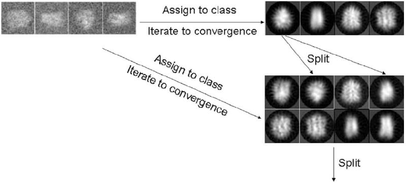
Divisive clustering: Experimental images are assigned to the current number of classes as in a standard multireference algorithm (note that in our algorithm we have changed the distance metric and the clustering criterion). When this process has converged, we split the current classes starting by the largest cluster. Then, we reassign the experimental images to the new set of classes. This process is iterated until the desired number of classes (not necessarily a power of 2) has been reached.
Alternatively, we could have started directly with the final number of class centers and let the clustering optimize the initial class centers (this is exactly how multireference alignment is usually applied in electron microscopy). However, this algorithm is known to get more easily trapped into local minima. Divisive clustering is less prone to local minima (Gray, 1984), although it is not guaranteed that the global minimum will be reached (this is a general drawback of K-means algorithms).
Our algorithm is an adaptation of this standard clustering algorithm to the cryo-EM setting. Since our main goal is recognizing the most common projections in the dataset, if at any moment a class represents less than a user given percentage of the total number of images (in the order of , being Nimg the total number of images and K the current number of classes), we remove that class from the quantization and split the class with the largest number of images assigned. Note that we do not remove the corresponding experimental images from the dataset. Instead, in the next quantization iteration, these images will be assigned to one of the remaining clusters.
2.3. Clustering criterion
Instead of using the L2 norm of the error to measure the similarity between an experimental image and a class representative, we propose to use the correntropy introduced earlier. Correntropies closer to 1 mean a larger agreement between the experimental image and the class representative.
Unfortunately, simply assigning an image to the class with highest correntropy does not result in a good classification of the images. The problem is that the absolute value of the correntropy is meaningless when comparing an experimental image to several classes (a similar problem has already been reported in electron microscopy using the correlation index (Sorzano et al., 2004a)). The reason for this is that at low Signal-to-Noise Ratios, the differences between two images may be absolutely masked by the noise, and the wrong assignment may be done simply because one class average is less noisy than another one. It could be said in this situation that the cleanest class “attracts” many experimental images even if they belong to some other class.
Let us prove this statement with a simple example. Let us presume that our experimental data comes from only two underlying classes A0 and A1, and that, after alignment, the experimental images are simply noisy versions of these two classes: Xi = Aj + Ni, where Xi is the ith experimental image, Aj is either A0 or A1, and Ni is a white noise image added during the experimental acquisition. Let us assume that at a given moment we have perfectly aligned and classified the experimental images in these two classes and that we have M0 images in the class generated by A0 and M1 images in the class generated by A1. Note that A0 and A1 are unknown (in fact, the multireference classification problem consists in estimating them), and all we have are estimates obtained by averaging the images assigned to each class, i.e., Âj = Aj + N̂j, where Âj are our estimates of the true underlying class averages and N̂j is some noise image obtained as the average of all the noise images of the experimental images assigned to this class. If the variance of the experimental images is σ2, then the variance of N̂j is .
The classical multireference clustering criterion is “Choose for Xi the class Aj that minimizes
where P is the total number of pixels, while Xip and Âjp denote the pth pixel of the experimental image and the class average, respectively. Let us assume that Xi really belongs to class A1, and let us see under which conditions it would be correctly assigned to class 1:
| (6) |
In other words, the experimental image will fail to be correctly classified unless the SNR of the difference between the two underlying classes is larger than a certain threshold (in electron microscopy images this is not always the case, as we try to capture very subtle differences in very noisy images). Let us further assume that there are many more images in A0 than in A1, i.e., is “negligible” versus , moreover M1 tends to be a small number and is particularly high. In other words, if one of the classes is large (M0 ≫ M1), Xi will fail to be assigned to its correct class and the class with more images assigned, A0, “attracts” many images from the other class.
Although we have presented the problem with the variance, this problem also occurs when using correntropy or maximum likelihood (Scheres et al., 2005). We propose an alternative clustering criterion that we will refer to as the robust criterion. Instead of looking only at the energy of the difference between the experimental image and the two estimates of the class averages, we propose to compare this energy to the energy of the rest of images compared to each class average. For instance, consider an experimental image whose correntropy with the representative of class A is 0.8, and with the representative of class B is 0.79. Because of the noise, these numbers cannot be blindly trusted and simply assign the experimental image to class A. Let us consider the correntropies of all images assigned to class A and of all images assigned to class B. If most correntropies of images in class A is in the order of 0.9, our image would be a very bad member of class A. However, if most correntropies of images in class B is in the order of 0.7, our image would be a very good member of class B (despite the fact that in absolute terms, the correntropy to class B is a little bit smaller than that to class A).
How good a correntropy is with respect to each one of these sets can be measured through the distribution functions
| (7) |
The first one measures the probability of having a correntropy smaller than a given value υ within the set of images assigned to class k. The second one measures the probability of having a correntropy smaller than a given value υ within the set of images not assigned to class k. The class to which an image Xi is assigned should be the one maximally fulfilling both goals
| (8) |
The classical clustering criterion is good for large differences between the class averages, while the robust clustering criterion is specially designed for subtle differences embedded in very noisy images. That is why we prefer to use this second criterion when splitting the nodes during the divisive clustering algorithm.
2.4. Final algorithm: CL2D
With the pieces introduced so far (correntropy, divisive clustering, and robust clustering criterion) we propose to use the following clustering algorithm that we will refer to as CL2D.
Algorithm 1. CL2D
Input:
S: Set of images
K0: Number of classes in the first iteration
KF: Number of classes in the last iteration
Output:
CKF : Set of KF class representatives
begin
// Initialize the classes
k = K0
Ck = Randomly split S into k classes
Update the distributions of Eq. (7)
σ2 = Measure the noise power in the background of the experimental images
// Refine the classes
Ck = Refine Ck with the data in S
-
while k < KF do
Cmin(2k, KF) = Split the largest min(k, KF – k) classes of Ck
k = min(2k, KF)
Ck = Refine Ck with the data in S
end
end
The refinement of the current classes is performed according to the following algorithm.
Algorithm 2. CL2D refinement of the current class representatives (Ck)
Input:
S: Set of images
Ck: Set of k class representatives
σ2: Noise power in the background of experimental images
Itermax: Maximum number of iterations
Nmin: Minimum number of images in a class
Output:
Ck: Refined set of k class representatives
begin
Iter = 0
-
repeat
// Assign all images to a class
-
foreach image ∈ S do
-
foreach classAverage ∈ Ck do
image =Align image to classAverage
Compute argument of Eq. (8)
end
Assign image to the class maximizing Eq. (8)
-
end
// Remove small classes and split the largest ones
-
while there are classes with less than Nmin images do
Remove the class with the smallest number of images assigned
Split the largest class of Ck
end
Update the distributions of Eq. (7)
Iter = Iter + 1
until No: of Changes < 0:5% and Iter < Itermax;
end
The split of a class is performed in a way very similar to that of the refinement of the current classes. The main difference is how the two subclasses are initially calculated. While in the standard algorithm these are computed by a random split, in the CL2D split we separate the images with the largest correntropies to the class average from the images with the smallest correntropies:
Algorithm 3. CL2D split of a class
Input:
S(c): Set of images assigned to class c
c: Class representative of class c
Output:
c1, c2: Two subclasses derived initially from class c
begin
// Split the images into two initial subclasses
c1 = Average of all images assigned to c with the largest 50%
correntropies
c2 = Average of all images assigned to c with the smallest 50%
correntropies
Update the distributions of Eq. (7) for these two subclasses
// Refine the two subclasses
Refine {c1, c2} with the data in S(c)
end
3. Results
To validate our algorithm we first performed a number of simulated experiments with the aim of testing the clustering approach to the multireference alignment problem. We used two different datasets for assessing the properties of the algorithm: one with the bacteriorhodopsin monomer to assess its clustering properties with respect to the projection point of view; and another with the Escherichia coli ribosome in two different conformational states to assess its clustering properties with respect to the conformational state. We then applied the algorithm to experimental data. In all the experiments we compared our results to those of ML2D (Scheres et al., 2005), SVD/MSA (script refine2d.py) in EMAN (Ludtke et al., 1999), Diday’s method, Hierarchical clustering and K-means from Spider (Frank et al., 1996) (scripts cluster.spi, hierarchical.spi, and kmeans.spi). Algorithms in Spider are preceded by a filtering and dimensionality reduction by Principal Component Analysis (PCA).
3.1. Simulated data: bacteriorhodopsin
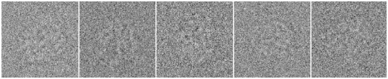
To test our algorithm we generated 10,000 projections randomly distributed in all projection directions from the bacteriorhodopsin monomer (PDB entry: 1BRD) and added white Gaussian noise with a SNR of 1/3 and 1/30 (see Fig. 2). We then applied our algorithm to compute 256 class averages with a maximum iteration count of 20. We found that this parameter is not critical as long as it is not too small so that the algorithm is stopped when the classes are not well established yet.
Figure 2.
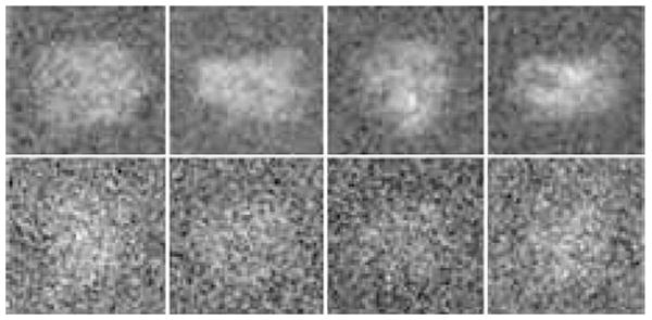
Simulated data: Sample noisy projections of the bacteriorhodopsin. Top row: the SNR is 1/3. Bottom row: the SNR is 1/30.
In our first experiment we tried to assess the effectiveness of each one of the three main modifications to the clustering algorithm (correntropy vs. correlation, divisive clustering vs. multireference clustering, classical clustering criterion vs. robust clustering criterion). For doing so, we conducted four experiments with the dataset with SNR = 1/3: the first one with the three new features (see its results in Supp. Fig. 1), and other three in which one of the new features was missing (correntropy, divisive clustering, or robust clustering). For each one of the experiments we evaluated each cluster by computing the angle between the projection directions of any pair of images assigned to that cluster. Finally, we computed the histogram of these angular distances in order to compare the different choices of the algorithm. Fig. 3 shows these histograms. It can be seen that the best combination is the one using two of the three new ideas introduced in this paper: correntropy and divisive clustering. As has already been mentioned before, this simply means that the SNR of the differences between classes is large enough to overcome the attraction effect (in the next subsection we present a case in which the robust clustering criterion performs better than the classical one because the input images have much lower SNR).
Figure 3.
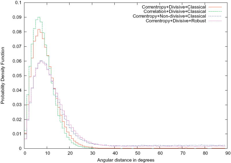
Clustering quality: probability density function estimate of the angular distance between projection directions of images assigned to the same cluster for the different execution modes of our clustering algorithm. Ideally, these functions should be concentrated at low angular distances meaning that the projections assigned to a cluster have similar projection directions. The maximum angular distance is 90° since the worse situation is that two orthogonal views (e.g. top and side views) are assigned to the same cluster.
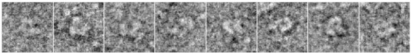
We repeated this experiment using ML2D (see Supp. Fig. 2). The algorithm could not produce more than 20 different classes that accounted for 97.1% of the particles (the algorithm was run with 50 classes, and the remaining 30 classes accounted only for 58 images, existing even empty classes). This result illustrates the “attractive” effect described during the introduction of the robust clustering criterion. Moreover, there was at least one class average (with 129 images assigned) in the ML2D approach that did not really represent any of the true projection images (see Fig. 4). In fact, if we analyze the 129 images assigned to this node with our algorithm, it can be seen that the ML2D class is actually a mixture of at least four different classes with 29, 35, 35, and 30 images, respectively.
Figure 4.
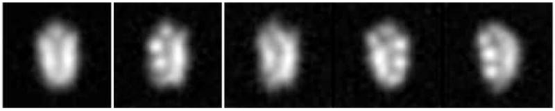
Example of a class wrongly identified by ML2D: The first image on the left is the class average found by ML2D (it represented 129 images from the original dataset). The other four images are classes found by CL2D applied to these 129 images. It reveals the existence of at least four different classes (with 29, 35, 35, and 30 images, respectively) within the set of 129 images assigned to a single class by ML2D.
We also repeated this experiment with SVD/MSA (classes not shown but we did not observe the “attraction” effect), PCA/Diday, PCA/Hierarchical, and PCA/K-means (with both dataset SNR = 1/3 and SNR = 1/30). As suggested in the multivariate data analysis web page of Spider (http://www.wadsworth.org/spider_doc/spider/docs/techs/MSA), we filtered our images with a Butterworth filter between the digital frequencies 0.25 and 0.33 (these frequencies are normalized in such a way that 1 corresponds to the Nyquist frequency). We also prealigned the images and reduced their dimensionality using a PCA with nine components. This preprocessing was applied to the data before using the three algorithms of Spider. In Fig. 5 we show the different estimates of the probability density function of the angular distance between the projection directions of images assigned to the same cluster for the six algorithms. It can be clearly seen that CL2D produces the tightest clusters in terms of projection directions.
Figure 5.
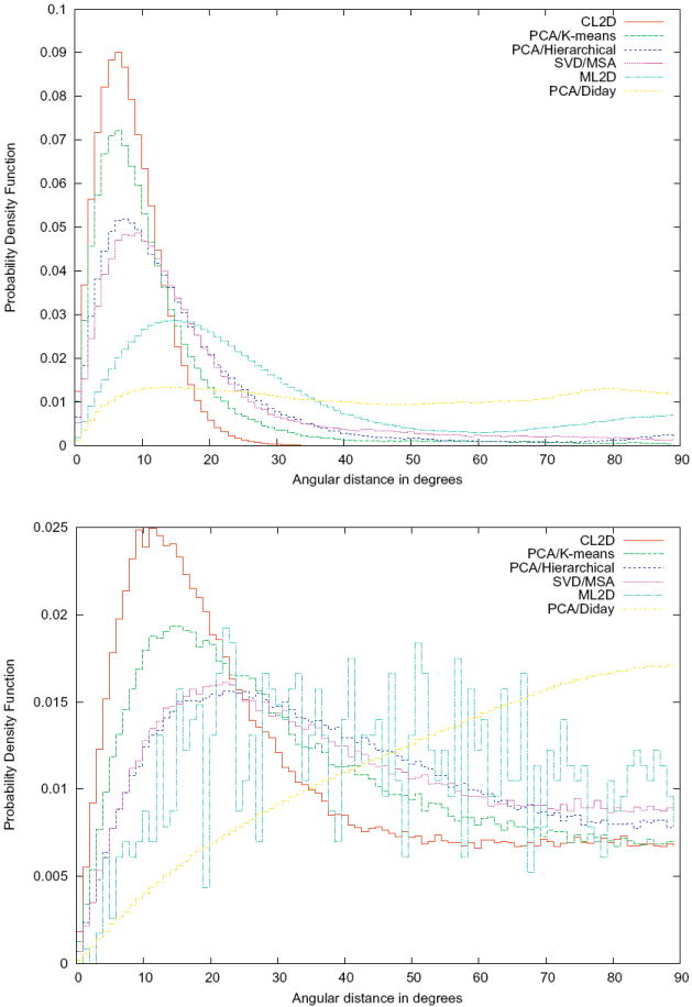
Clustering quality: probability density function estimate of the angular distance between projection directions of images assigned to the same cluster for six different clustering algorithms (top, SNR = 1/3; bottom SNR = 1/30).
The execution times in a single CPU (Intel Xeon 2.6 GHz) for PCA/Diday, PCA/Hierarchical and PCA/K-means was about 0.3 h, 50 h for SVD/MSA, 100 h for CL2D, and 74 h for ML2D (with only 64 classes; CL2D took 41 h in computing 64 classes). However, CL2D has been parallelized with MPI and has been run in parallel with 32 nodes, reducing the computation time to 3.5 h.
The experiment was repeated in a more realistic setup by introducing the effect of the microscope Contrast Transfer Function (CTF) with an acceleration voltage of 200 kV, a defocus of −5.5 μm, and a spherical aberration of 2.26 mm. Results were similar to the previous case (results not shown).
3.2. Simulated data: E. coli ribosome
For this test we used the public dataset of simulated ribosomes available at the Electron Microscopy Data Bank (http://www.ebi.ac.uk/pdbe/emdb/singleParticledir/SPIDER_FRANK_data, (Baxter et al., 2009)). This dataset contains 5000 projections from random directions of a ribosome bound with three tRNAs at A, P, and E sites, and other 5000 projections from random directions of an EF-G(GDPNP)-bound ribosome with a deacylated tRNA bound in the hybrid P/E position. Besides these differences in the ligands, these two ribosomes also have different ribosomal conformations: the first ribosome is in the normal conformation, while the second ribosome is in a ratcheted configuration (30S subunit rotated counter-clockwise relative to the 50S subunit). Fig. 6 shows some sample images from this dataset.
Figure 6.
Simulated data: Sample noisy projections of the ribosome in two different conformations.
The goal of this experiment is to characterize the capability of the new algorithm to separate the two conformational states, i.e., to produce classes in which the majority of the images assigned comes from the same conformational state.
With our previous dataset we already showed the superiority of the correntropy over correlation, and of the divisive clustering over a classical multireference clustering. In the previous dataset it also appeared that the classical clustering criterion was superior to the robust clustering criterion. However, as was already discussed in the Methods Section, this holds for sufficiently high SNRs. This dataset has a much lower SNR than the previous one. We ran our algorithm to partition the input data into 256 classes using the classical clustering criterion and the new robust criterion. For each class we tested the hypothesis that the two ribosomes were equally represented (the proportion of images of each type was 0.5). The classical clustering criterion only found 67 classes (out of 256) where the proportion of the majority of the images were significantly different (with a 95% of confidence) from 50%. The amount of images assigned to these classes was 2822. However, the new robust clustering criterion was able to identify 98 classes where the majority of images significantly came from a single ribosome type. The amount of images assigned to these 98 classes was 4130. The difference between the proportions of classes with a majority of ribosomes of one type using the classical and the robust clustering criteria was significantly different with a confidence of 95%.
We repeated the same experiment with SVD/MSA, ML2D, PCA/Diday’s clustering, PCA/Hierarchical clustering and PCA/K-means. SVD/MSA identified 107 classes with a statistically significant majority of images of one type (4534 images were assigned to these classes). However, the difference between the proportions of SVD/MSA and CL2D was not statistically significant with a confidence level of 95%. ML2D identified 9 classes with a statistically significant majority of images of one type (1439 images were assigned to these classes). Images were preprocessed in exactly the same way as in the previous experiment before applying any of Spider’s methods. PCA/Diday method produced 11 classes with a statistically significant majority of images of one type (899 images were assigned to these classes). The PCA/Hierarchical clustering produced 74 classes with a statistically significant majority of images of one type (with 3049 images assigned to them). The PCA/K-means produced 53 classes with a statistically significant majority of images of one type (with 2114 images assigned to them).
3.3. Experimental data: p53
We applied our algorithm to a dataset that contained 7600 projections of a mutant of p53 without the C-terminal domain bound to the GADD45 DNA sequence (Ma et al., 2007; Tidow et al., 2007). The sample was negatively stained. The pixel size was 4.2 Å/pixel and the image size was 60 × 60 pixels (see Fig. 7). We applied our algorithm to generate 256 class averages (20 iterations per Hierarchical level). Supp. Fig. 3 shows the resulting classes. In an experimental setting it is difficult to validate the 2D classes produced by an algorithm. In this experiment at least we tested that the classes produced captured enough information from the original dataset. For doing so, we built a reference volume based on the common lines of the classes produced by CL2D (see Fig. 8a). This reference volume was refined in two different ways: first, using the CL2D classes themselves as the only projections in the dataset (the refined volume is shown in Fig. 8b); second, using the whole dataset of projections (the refined volume is shown in Fig. 8c). Interestingly, the volumes in Fig. 8b and c are consistent with each other up to 32 Å (at this frequency the Fourier Shell Correlation (Harauz and van Heel, 1986) between the two volumes drops below 0.5). Considering that the resolution of the volume in Fig. 8c is around 27 Å, the approximation up to 32 Å of the volume reconstructed using only the CL2D classes is not a bad approximation. The same projection dataset was refined using a reference volume obtained independently through Random Conical Tilt (Scheres et al., 2009).
Figure 7.
Examples of the experimental images: Sample projections of the p53 mutant.
Figure 8.
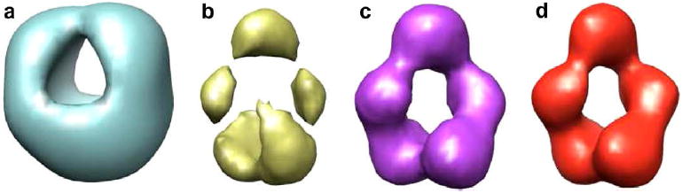
Reconstructions of p53: Isosurface representation containing 100% of the protein mass of a mutant of p53 without the N-terminal domain bound to DNA. (a) Reconstructed from the CL2D classes using common lines. (b) Refinement of the volume in a) using only the CL2D classes. (c) Reconstruction performed from the whole dataset using the volume obtained in (a) as the starting reference. (d) Reconstruction performed from the whole dataset but using a volume obtained by Random Conical Tilt as the starting reference.
4. Discussion
In this paper we have introduced a new multireference alignment algorithm that can be briefly explained as follows. If we think of projection images of size N × N as vectors in a N2-dimensional space, we can define our algorithm as one that looks for N2-dimensional points trying to be close to the distribution of points corresponding to the original images in this space. This is exactly the goal of vector quantization or clustering. Close or distant images are defined using the correntropy, a similarity function that has been proved to be useful for non-Gaussian noise sources; while the clustering criterion has been modified to a robust version in order to be able to overcome the “attraction” effect affecting the any clustering criterion based on a term similar to that of minimum variance. Summarizing, the four key ideas of our algorithm are:
Use of correntropy as a similarity measure between images instead of the standard least-squares distance or, its equivalent, cross-correlation. Correntropy has proven to be an useful similarity measure in non-linear, non-Gaussian signal processing and it has been related to the M-estimates of robust statistics.
Use of clustering as a means of producing many classes with a small amount of images in each class. In this way we have a better angular coverage of the projection sphere and avoid averaging too many images in the same cluster.
Use of a divisive algorithm for performing the clustering as a means of avoiding getting trapped in a local minimum of the quantization problem. Although global convergence is not guaranteed, it has been shown (Gray, 1984) that experimentally, divisive clustering is more robust than a clustering attempting to directly produce the final number of class averages.
The assignment of an image to one class is not performed by simply choosing the class with maximum correntropy. We found that this simple strategy leads to a reduced number of “attractive” classes if the SNR of the differences to be detected is not sufficiently large. Alternatively, we propose to compare for each class, the correntropy of the image at hand, the set of correntropies of all the images assigned to that class, and the set of correntropies of all the images not assigned to that class. Then, we choose the class that maximizes the probability of being better than all the images assigned and being better than all the images not assigned.
We have tested this algorithm with a number of simulated and experimental datasets. In the simulated datasets we found that our algorithm is much better suited than ML2D, SVD/MSA, PCA/Diday, PCA/Hierarchical and PCA/K-means to discover many different projection directions. ML2D suffered from “attractor” classes, i.e., the algorithm was unable of working with many output reference classes (many of the classes are empty or nearly empty). This cannot happen in our algorithm by its construction: when a class is too small (represents less than a user-specified percentage of the input images), the class is removed and the largest class will be splitted in two. The few images assigned to the removed representative have to find a new representative in the next iteration. Using a sufficiently large number of class representatives, it is expected to better represent the input dataset. In fact, this is what we actually observed using the histogram of angular differences between pairs of images assigned to the same cluster (the angular difference between two images is defined as the difference in degrees between their projection directions). In our first experiment with simulated data, we observed that the combination of correntropy, divisive clustering, and classical clustering criterion was the one producing the best results. Changing any of these three features resulted in lower performance. However, in our second experiment we showed that the classical clustering criterion is not always the most successful. The second dataset had a much lower SNR and, as expected, the newly introduced robust clustering criterion overperformed the classical criterion.
In our first simulated dataset we also discovered that some of the classes returned by ML2D could be understood as a mixture of several other classes. The problem of handling many classes seems to be attenuated in the SVD/MSA, PCA/Hierarchical and PCA/K-means approaches. However, we have already shown that our algorithm is able of producing tighter clusters in terms of projection directions and, therefore, it is more likely to achieve good common line reconstructions. With our experiment with the p53 mutant we have shown that reference volumes constructed by common lines from our CL2D classes are capable of being refined to yield a volume that is similar to one obtained by starting from a Random Conical Tilt data collection. Moreover, the refinement of the initial volume constructed with common lines using only our CL2D classes is able to produce a volume that is compatible with the best reconstruction of this dataset up to 32 Å (the resolution of the best reconstruction is around 27 Å).
When clustering images with different projection directions and belonging to different conformational states (the ribosomal simulated data), our algorithm was able to generate a proportion of classes with a majority of images from a single ribosome type that was not significantly different from the same proportion in case of using SVD/MSA, and significantly better than ML2D, PCA/Diday, the PCA/Hierarchical and the PCA/K-means. We could not evaluate the angular spread of each one of the classes because this information is missing in this standard benchmark.
5. Conclusions
In this paper we have introduced a new algorithm for two-dimensional multireference alignment. It is based on the idea of creating many classes with a small number of images assigned to each class in order to avoid too much averaging. Moreover, we have used correntropy as the similarity function, a recently introduced alternative to cross-correlation which is sensitive to non-Gaussian noise sources and is related to robust statistics. We have also introduced a new clustering criterion that in our experiments did not suffer from the “attraction” problem even at low SNR. We have proven that this algorithm can be successfully applied to electron microscopy images of single particles producing higher-quality results than those of the most widely used algorithms in the field. This algorithm is freely available from the Xmipp software package (Sorzano et al., 2004b; Scheres et al., 2008) (http://xmipp.cnb.csic.es).
Supplementary Material
Acknowledgments
The authors are thankful to Dr. Scheres for revising the final manuscript and for insightful discussions, and to Dr. Martín-Benito for his help running the Spider algorithms. This work was funded by the European Union (projects FP6-502828 and UE-512092), the 3DEM European network (LSHG-CT- 2004-502828) and the ANR (PCV06-142771), the Spanish Ministerio de Educación (CSD2006-0023, BIO2007-67150-C01 and BIO2007-67150-C03), the Spanish Ministerio de Ciencia e Innovación (ACI2009-1022), the Spanish Fondo de Investigación Sanitaria (04/0683) and the Comunidad de Madrid (S-GEN-0166-2006). The authors wish to thank support from grants MCI-TIN2008-01117 and JA-P06-TIC01426. J.R. Bilbao-Castro is a fellow of the Spanish “Juan de la Cierva” postdoctoral contract program, co-financed by the European Social Fund. C.O.S. Sorzano is a recipient of a “Ramón y Cajal” fellowship financed by the European Social Fund and the Ministerio de Ciencia e Innovación. G. Xu was supported in part by NSFC under the grant 60773165, NSFC key project under the grant 10990013. The project described was supported by Award Number R01HL070472 from the National Heart, Lung, And Blood Institute. The content is solely the responsibility of the authors and does not necessarily represent the official views of the National Heart, Lung, And Blood Institute or the National Institutes of Health. The funders had no role in study design, data collection and analysis, decision to publish, or preparation of the manuscript.
Footnotes
Appendix A. Supplementary data Supplementary data associated with this article can be found, in the online version, at doi:10.1016/j.jsb.2010.03.011
References
- Baxter WT, Grassucci RA, Gao H, Frank J. Determination of signal-to-noise ratios and spectral snrs in cryo-em low-dose imaging of molecules. J Struct Biol. 2009 May;166(2):126–132. doi: 10.1016/j.jsb.2009.02.012. [DOI] [PMC free article] [PubMed] [Google Scholar]
- Chong CW, Raveendran P, Mukundan R. Translation invariants of zernike moments. Pattern Recogn. 2003;36:1765–1773. [Google Scholar]
- Dempster A, Laird N, Rubin D. Maximum likelihood from incomplete data via the EM algorithm. J Roy Stat Soc, Ser B. 1977;39:1–38. [Google Scholar]
- Flusser J, Zitova B, Suk T. Invariant-based registration of rotated and blurred images. Proceedings of the Geoscience and Remote Sensing Symposium. 1999;2:1262–1264. [Google Scholar]
- Frank J, Radermacher M, Penczek P, Zhu J, Li Y, Ladjadj M, Leith A. SPIDER and WEB: processing and visualization of images in 3D electron microscopy and related fields. J Struct Biol. 1996;116:190–199. doi: 10.1006/jsbi.1996.0030. [DOI] [PubMed] [Google Scholar]
- Gray RM. Vector quantization. IEEE Acoust Speech Signal Process Mag. 1984;1:4–29. [Google Scholar]
- Harauz G, van Heel M. Exact filters for general geometry three dimensional reconstruction. Optik. 1986;73:146–156. [Google Scholar]
- Liu W, Pokharel PP, Prfncipe JC. Correntropy: properties and applications in non-gaussian signal processing. IEEE Trans Signal Process. 2007;55:5286–5298. [Google Scholar]
- Lowe D. Object recognition from local scale-invariant features. Proceedings of the ICCV. 1999:1150–1157. [Google Scholar]
- Lowe DG. Distinctive image features from scale-invariant keypoints. Int J Comput Vis. 2004;60:91–110. [Google Scholar]
- Ludtke SJ, Baldwin PR, Chiu W. EMAN: semiautomated software for high-resolution single-particle reconstructions. J Struct Biol. 1999;128:82–97. doi: 10.1006/jsbi.1999.4174. [DOI] [PubMed] [Google Scholar]
- Ma B, Pan Y, Zheng J, Levine AJ, Nussinov R. Sequence analysis of p53 response-elements suggests multiple binding modes of the p53 tetramer to dna targets. Nucleic Acids Res. 2007;35:2986–3001. doi: 10.1093/nar/gkm192. [DOI] [PMC free article] [PubMed] [Google Scholar]
- Marabini R, Carazo JM. Practical issues on invariant image averaging using the bispectrum. Signal Process. 1994;40:119–128. [Google Scholar]
- Pun CM. Rotation-invariant texture feature for image retrieval. Comput Vis Image Underst. 2003;89:24–43. [Google Scholar]
- Santamarfa I, Pokharel PP, Prfncipe JC. Generalized correlation function: definition, properties, and application to blind equalization. IEEE Trans Signal Process. 2006;54:2187–2197. [Google Scholar]
- Schatz M, van Heel M. Invariant classification of molecular views in electron micrographs. Ultramicroscopy. 1990;32:255–264. doi: 10.1016/0304-3991(90)90003-5. [DOI] [PubMed] [Google Scholar]
- Schatz M, van Heel M. Invariant recognition of molecular projections in vitreous ice preparations. Ultramicroscopy. 1992;45:15–22. [Google Scholar]
- Scheres SH, Melero R, Valle M, Carazo JM. Averaging of electron subtomograms and random conical tilt reconstructions through likelihood optimization. Structure. 2009;17:1563–1572. doi: 10.1016/j.str.2009.10.009. [DOI] [PMC free article] [PubMed] [Google Scholar]
- Scheres SHW, Nuśez-Ramfrez R, Sorzano COS, Carazo JM, Marabini R. Image processing for electron microscopy single-particle analysis using xmipp. Nat Protoc. 2008;3:977–990. doi: 10.1038/nprot.2008.62. [DOI] [PMC free article] [PubMed] [Google Scholar]
- Scheres SHW, Valle M, Núñez R, Sorzano COS, Marabini R, Herman GT, Carazo JM. Maximum-likelihood multi-reference refinement for electron microscopy images. J Mol Biol. 2005;348:139–149. doi: 10.1016/j.jmb.2005.02.031. [DOI] [PubMed] [Google Scholar]
- Schmid C, Mohr R. Local greyvalue invariants for image retrieval. IEEE Trans Pattern Anal Mach Intell. 1997;19:530–535. [Google Scholar]
- Sorzano COS, Jonic S, El-Bez C, Carazo JM, De Carlo S, ThTvenaz P, Unser M. A multiresolution approach to pose assignment in 3-D electron microscopy of single particles. J Struct Biol. 2004a;146:381–392. doi: 10.1016/j.jsb.2004.01.006. [DOI] [PubMed] [Google Scholar]
- Sorzano COS, Marabini R, Velázquez-Muriel J, Bilbao-Castro JR, Scheres SHW, Carazo JM, Pascual-Montano A. XMIPP: a new generation of an open-source image processing package for electron microscopy. J Struct Biol. 2004b;148:194–204. doi: 10.1016/j.jsb.2004.06.006. [DOI] [PubMed] [Google Scholar]
- Tidow H, Melero R, Mylonas E, Freund SMV, Grossmann JG, Carazo JM, Svergun DI, Valle M, Fersht AV. Quaternary structures of tumor suppressor p53 and a specific p53 dna complex. Proc Natl Acad Sci USA. 2007;104:12324–12329. doi: 10.1073/pnas.0705069104. [DOI] [PMC free article] [PubMed] [Google Scholar]
- Tuytelaars T, Van Gool L. Content-based image retrieval based on local affinely invariant regios. Vis Inform Inform Syst. 1999:493–500. [Google Scholar]
- van Heel M, Stoffler-Meilicke M. Characteristic views of E. coli and B. staerothermophilus 30s ribosomal subunits in the electron microscope. EMBO J. 1985;4:2389–2395. doi: 10.1002/j.1460-2075.1985.tb03944.x. [DOI] [PMC free article] [PubMed] [Google Scholar]
Associated Data
This section collects any data citations, data availability statements, or supplementary materials included in this article.