Abstract
Motivation: Recently, structural genomic variants have come to the forefront as a significant source of variation in the human population, but the identification of these variants in a large genome remains a challenge. The complete sequencing of a human individual is prohibitive at current costs, while current polymorphism detection technologies, such as SNP arrays, are not able to identify many of the large scale events. One of the most promising methods to detect such variants is the computational mapping of clone-end sequences to a reference genome.
Results: Here, we present a probabilistic framework for the identification of structural variants using clone-end sequencing. Unlike previous methods, our approach does not rely on an a priori determined mapping of all reads to the reference. Instead, we build a framework for finding the most probable assignment of sequenced clones to potential structural variants based on the other clones. We compare our predictions with the structural variants identified in three previous studies. While there is a statistically significant correlation between the predictions, we also find a significant number of previously uncharacterized structural variants. Furthermore, we identify a number of putative cross-chromosomal events, primarily located proximally to the centromeres of the chromosomes.
Availability: Our dataset, results and source code are available at http://compbio.cs.toronto.edu/structvar/
Contact:seunghak@cs.toronto.edu,echeran@cs.toronto.edu,brudno@cs.toronto.edu
1 INTRODUCTION
One of the fundamental problems in bioinformatics is the discovery of the genomic variation present within the human population, and the association between these genotypes and phenotypes. Initially, it was thought that the bulk of variation between individuals were point mutations (SNPs). However, as the HapMap project (The International HapMap Consortium, 2003) has increased our understanding of SNPs, it has also identified large-scale structural genomic variation, including insertions, deletions, translocations, inversions and copy number variants (CNVs) (Iafrate et al., 2004) as equally significant sources of differences between individual genomes. A wide variety of methods have been used to find these events (Feuk et al., 2006): for CNVs, for example, microarray technologies are capable of detecting significant differences in copy number between two DNA samples using comparative genome hybridization (CGH) techniques (Kallioniemi et al., 1992); (Lucito et al., 2003).
These methods, while useful for finding duplications, do not detect ‘balanced’ structural changes—those that do not result in a change in the abundance of DNA that matches any probe, such as inversions and translocations. Recently, the completion of the diploid genome of an individual (Levy et al., 2007) has, for the first time, made it possible to directly compare two complete human genomes, enabling us to begin to understand the variety of genotypes present in the human population. This fully assembled genome, however, is quite different from the data that will become available in the near future. The National Human Genome Research Institute is planning to sequence the genomes of 1000 human individuals in the next few years using next generation sequencing (NGS) technologies. While the NGS technologies will drastically reduce the cost of resequencing an individual human, it is currently unclear to what extent these platforms can be used to identify structural variations.
The bulk of the currently known structural variants have been determined by mapping either individual reads (Mills et al., 2006) or clone-ends (Korbel et al., 2007; Tuzun et al., 2005) from donor individuals to a reference genome. Many sequencing techniques allow for the generation of reads from the two ends of a DNA fragment simultaneously. Because the size of a DNA fragment can be determined, e.g. by running it on a gel, this allows for the generation of paired reads, positioned at a known distance (insert size) from each other in a genome. Such pairs of reads are known as clone-ends, or matepairs. Using a known genomic sequence as a reference, matepairs can be used to locate structural variations. To locate potential areas of rearrangements, one first maps a matepair to this reference. If the size of the insert differs significantly from the distance between the mapped positions on the genome (the matepair is discordant), then the implication is that there is a variation at this locus or that there is an error in either the sequenced insert, or the reference genome. While one may assume that the reference genome is accurate, errors in insert size estimation and assigning locations to the reads make the determination of structural variants from clone-end data non-trivial.
Tuzun and colleagues conducted the original study of applying clone paired-end sequencing to find putative locations of insertions, deletions and inversions (Tuzun et al., 2005). They concentrated on the analysis of reads from a single human donor. Reads were mapped to the genome, but any read that mapped to a known recent segmental duplication was removed from consideration. If a read mapped to multiple possible locations on the genome, a simple set of rules was followed, favoring hits that mapped at a distance equal to the length of the insert and those that had a higher degree of similarity. All inserts for which the mapped distance between the reads was within 3 standard deviations of the mean were discounted as not having enough statistical significance to identify a structural variant. The authors identified inversions whenever clone ends did not map in opposite orientations. Matepairs that mapped further than 10 Mb from each other, or to locations on different chromosomes, were discarded. Because of potential errors in clone construction and read mapping, rearrangements were identified only when two distinct clones supported it. In the study, they identified 297 potential variants. A similar approach was used in a recent study by Korbel et al., (2007), with the main difference being the use of 454 sequencing technology with a smaller insert size. They identified 881 structural variants based on the genomes of two donor individuals.
The use of NGS technology will make the computational problem of finding variations using clone-end data more challenging. The short (25–50 bp) reads generated by NGS platforms will often not map uniquely onto the reference genome. Consequently, it is necessary to develop methods for detecting structural variants using clone-ends without reliable mappings. Both the approaches of Tuzun et al., (2005) and Korbel et al., (2007) attempt to assign a priori every clone-end to some location on the genome, an approach that is unlikely to scale if every read maps to a large number of different locations. Here we present an alternative approach, where we consider all possible mappings for each read, and assign each read to a location based not only on that read, but also based on all of the other reads generated from the dataset. Furthermore, we explore the use of concordant matepairs to identify heterozygous and homozygous events and control the false discovery rate via a corrected P-value. We use our method to identify structural variations between the recently published diploid human genome Levy (et al., 2007) and the public reference genome Lander (et al., 2001). Our results, while significantly correlated with previously known variants, also include a large number of putative novel events.
2 METHODS
In this article, we describe a method to predict structural variations, including insertions, deletions, inversions and translocations using a probabilistic framework. Our method follows the general approach of Tuzun et al., (2005), where clone-end sequences from one individual are compared to a reference genome. If the mapped distance of a matepair is significantly different from the insert size of the matepair, then we may speculate that there is an insertion or a deletion (indel) between the pair of reads of the matepair. If the two reads of a matepair map to the genome with the same orientations, this indicates an inversion. Finally, matepairs mapping to different chromosomes indicate cross-chromosomal events, which we refer to as translocations (these can also be explained by other means, see Section 3.3). In contrast to the Tuzun approach, which discarded clones mapping to recent segmental duplications and considered only a single best placement for every clone-end on the genome, we use a local search algorithm to find an assignment of each clone to a genomic locus, where our confidence in a particular assignment grows if other clones are mapped nearby.
2.1 Notation
In the method described below, we will make use of the following notation:
1. Let X1, X2, …, XN be the matepairs (clones), generated from the donor genome A, where N is the total number of matepairs. These are mapped to the reference genome REF.
2. Each matepair has two clone-ends, which are referred to as the forward and reverse reads. For a particular matepair, if the two reads are mapped to the reference genome in α and β positions, there exist M=α · β mapped positions for the matepair. The i-th mapped position for the matepair Xt is referred to as bi(Xt), where 1≤i≤M and 1≤t≤N.
3. The size of the insert between the two reads (the distance between them in the donor genome) for the matepair Xt is referred to as s(Xt). In a typical sequencing project, clones with varying insert lengths are generated.
4. A set of mapped locations of matepairs that explain the same structural variation is referred to as a cluster. We will build the set of clusters denoted by {C1, C2, …, CK}, where K is the number of clusters via hierarchical clustering.
- 5. The probability that the mapped location bi(Xt) ‘explains’ the same variant as the cluster Ck is denoted as P(bi(Xt)|Ck). For simplicity, we will write P(Xt|Ck) when the meaning is clear. We consider all matepairs to be independent, so the probability of two reads being a part of the same cluster P(Xi, Xj|Ck) is computed as

6. The probability that Ck is a genuine cluster explaining a real structural variant is denoted by P(Ck).
7. The probability that Ck is a genuine cluster given bi(Xt) is denoted by p(ck∣bi(xt). Again, we will use P(Ck|Xt) if the meaning is clear.
2.2 Probabilistic framework for structural variants
In the following four subsections, we will describe the probabilistic frameworks for four types of structural variants: insertions, deletions, inversions and translocations. For insertions and deletions, we define these relative to the reference genome: an insertion indicates the presence of a segment in the donor sample that is not in the reference. Conversely, a deletion implies a segment present in the reference that is not in the donor. Our framework does not capture more complex scenarios, such as those resulting from several events at a single locus.
We will rely on the observed probability distribution, p(Y), which indicates the likelihood of observing a given mapped distance for a particular insert size. This distribution is computed using those matepairs whose forward and reverse reads map uniquely to the reference genome, as they are the most reliable. Mapped distances greater than twice the insert size are not taken into account. Figure 1 shows the distributions p(Y) for insert sizes 10 000, 12 500, 43 000, and 45 000 in our dataset (Levy et al., 2007).
Fig. 1.
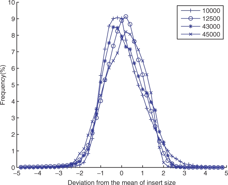
Probability distribution p(Y) of mapped distances for insert sizes. Zero is the mean of all of the distributions, and each unit on the x-axis is one standard deviation from the mean. The y-axis is the observed frequency of the corresponding mapped distances.
2.2.1 Insertion
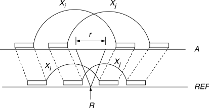
Figure 2 shows a pair of matepairs (Xi, Xj), both of which support an insertion of length r in genome A. When matepairs in the sampled genome A are mapped to the genome REF, the mapped distance of Xi and Xj decreases by r, because the corresponding segment is missing inbreak genome REF.
Fig. 2.
Matepairs Xi and Xj from the sample genome A are mapped to the reference genome REF. The size of insertion in genome A is r, thus the mapped distance of Xi and Xj in genome REF is decreased by r. R is the point where insertion took place.
If Xi and Xj are members of a cluster Ck, we wish to compute P(Xi, Xj|Ck), the probability that both Xi and Xj explain the insertion in Ck. First, note that the point R, where the insertion occurs, should be located in between the forward and reverse reads of both Xi and Xj. Otherwise, P(Xi, Xj|Ck)=0 as Xi and Xj cannot both explain the same insertion. Using the independence assumption (Section 2.1) and the probability distribution p(Y) explained above, we compute P(Xi,Xj|Ck)=P(Xi|Ck)P(Xj|Ck), as follows:
where μY is the mean of p(Y) and s is the mapped distance of Xi in genome REF. We determine r by maximizing P(Xi, Xj|Ck):
The key idea is that given the cluster Ck, r is the length of the insertion that is missing in genome REF. Thus, in the donor genome A, Xi has insert size of s+r, which should be close to the average insert size of matepairs. Because p(Y) is the observed distribution of insert sizes for inserts of size s(Xi), our formula computes the likelihood that a given read in the cluster was generated from a donor genome A that has an extra DNA segment of size r. Note that we will be unable to detect insertions of size larger than the insert size of the matepair.
2.2.2 Deletion
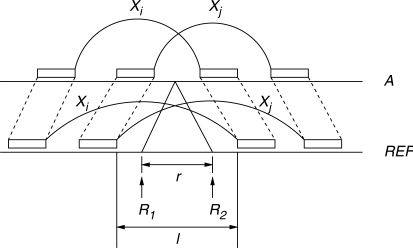
Figure 3 shows the case of a deletion with a cluster Ck and matepairs Xi and Xj. The deletion case is simply the opposite of the insertion, where the mapped distance in genome REF increases because of the deletion of size r in genome A.
Fig. 3.
Two matepairs, Xi and Xj, are mapped onto the reference genome REF. The mapped distances of Xi and Xj increase by r because of the deletion in the donor genome A. The length of overlap between Xi and Xj is l in the reference genome. The length of the deletion r should be less than or equal to l. R1 and R2 denote the points at which the deletion occurred.
Similar to the insertion, P(Xi, Xj|Ck)=0 if the two points R1 and R2 are not within the mapped positions of both Xi and Xj. Otherwise, we compute the probability of P(Xi, Xj|Ck) by again, using the independence assumption and distribution p(Y):
where μY is the average of p(Y) and δ=|μY − (s−r)|. Note that here, r is subtracted from s because the insert size of Xi in genome A is s−r assuming that there is a deletion of size r in genome A. The length of the deletion, r, associated with Ck is determined by maximizing P(Xi, Xj|Ck):
As shown in Figure 3, l is the length of the overlap between Xi and Xj in genome REF. Also, 0≤r≤l since the length of the deletion cannot exceed the length of the overlap l.
2.2.3 Inversion
Figure 4 shows an inversion with Xi and Xj in Ck. To be able to explain an inversion in genome A, both forward and reverse reads should have the same orientation when they are mapped to genome REF. Furthermore, all of the reads in a cluster should map to the same strand of the REF genome.
Fig. 4.
Two matepairs Xi and Xj lie on the region {R1, R2}, where an inversion has taken place. Note that the region {R1, R2} is flipped over, and the order of the right reads of Xi and Xj is reversed in genome REF.
In order to identify which matepairs are potentially in the same cluster, we note that the following equality holds if Xi and Xj are involved in the same inversion:
where c and d are the length between the start positions of the forward and reverse reads of Xi and Xj, as shown in Figure 4, and s(Xi) and s(Xj) are the known insert sizes of Xi and Xj in genome A. We can see that the above equality holds by inverting the region {R1, R2} as follows:
 |
In order to compute the probability P(Xi, Xj|Ck) for the case of inversions, we build the probability distribution p(|Y1−Y2|) using p(Y1) and p(Y2), which are the distributions of mapped distances for s(Xi) and s(Xj) sized matepairs, respectively:
where μ|Y1−Y2| is the average of p(|Y1−Y2|) and γ=|μ|Y1−Y2|−(c−d)|.
According to the above equation, for the case when the two matepairs Xi and Xj have the same insert size, if μ|Y1−Y2|=(c−d)=0, then P(Xi, Xj∣Ck)=1. Thus, the probability of the inversion is maximized when the reads that support it are most in agreement with each other. Here again, we assume that the mapped positions of Xi and Xj overlap on the REF genome. Otherwise, P(Xi, Xj|Ck)=0 because they cannot explain the same inversion.
Additionally, inverted matepairs can be used to estimate the length of the inverted region: consider the matepair Xj in Figure 4. Let m=b1+z−b2 be the distance between the mapped positions of the two reads in the reference genome. Because the inversion has flipped the mapped position around the midpoint of the [R1, R2] region, the size of the inversion must be m−s(Xj)<R2−R1<m+s(Xj). We will use the predicted insert size of all matepairs to identify opposite ends on inversions in Section 2.4.1.
2.2.4 Translocation
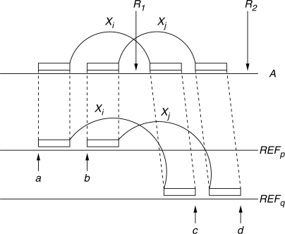
Figure 5 shows the case of a translocation with a cluster consisting of Xi and Xj matepairs, where the region {R1, R2} is translocated from chromosome p to chromosome q. There are two possible ways of mapping matepairs of genome A into REF. First, if we orient chromosomes p and q so that they have the same orientation, as shown in the figure, then the following conditions describe agreeing matepairs for a translocation:
where a, b, c and d refer to the points in Figure 5. The first equation implies that the difference between the mapped distances of matepair Xi and Xj are preserved. The second and third constraints mean that Xi and Xj should overlap to explain the same translocation.
Fig. 5.
This figure shows a translocation. One read of both matepairs Xi and Xj is mapped on chromosome p, and the other on chromosome q in genome REF. The region {R1, R2} is translocated and mapped onto chromosome q in genome REF with the same orientation.
The probability P(Xi, Xj|Ck) is defined as follows:
where χ=|μ|Y1−Y2|−{(c−a)−(d−b)}|.
Here, P(Xi, Xj|Ck)=0 if |b−a|>s(Xi) or |d−c|>s(Xj). In such a case, Xi and Xj do not overlap and they cannot be involved in the same translocation. It is also possible that the chromosomes p and q are oriented with opposite orientations. In this case, we need to reverse the coordinate system of chromosome q (e.g. the end of the chromosome becomes position one, while the beginning is now the end), but the rest of the calculations are unchanged.
2.3 Use of concordant matepairs
One important source of information that was not utilized in either the Tuzun et al., (2005) or the Korbel et al., (2007) studies is the presence of concordant matepairs (those mapping at approximately the expected insert size) near a cluster of discordant matepairs. These concordant matepairs are used by us for two analyses: determining, for each structural variant, if it is likely to be homozygous, and computing, for insertion and deletion clusters, the likelihood that they were generated by chance (P-value).
These analyses will rely on the number of concordant and discordant inserts mapped to the location of some cluster Ck. The number of discordant reads is taken as |Ck|. For computing the number of concordant matepairs we consider the cluster to have two halves, in which the left and right ends of the discordant reads map. Note that the two halves are not necessarily adjacent: for example, in Figure 5 the two halves are between a and b on chromosome p and c and d on chromosome q. The number of concordant matepairs is computed as the average of the number of left ends of concordant matepairs that map within the left half of the cluster, and right ends that map within the right end. If a particular matepair has k (concordant) mapped positions, then we count it as 1/k of a matepair when computing the number of concordant matepairs mapped to any cluster.
2.3.1 Determining heterozygosity
Deciding if a particular structural variant is heterozygous or homozygous is challenging when the total number of matepairs supporting the variant is small. When we observe a small number of discordant matepairs and no concordant ones, it is still possible that the variant is heterozygous, but no concordant matepairs were sequenced from the region. If we observe a small number of concordant matepairs in an otherwise discordant region, these could represent mismapped matepairs, or matepairs that end before the predicted breakpoint (often we can only determine a range in which the breakpoint occurred, rather than an exact location). We annotate a cluster as homozygous if it satisfies the following criteria: (1) no more than one uniquely mapped concordant matepair, (2) at least 4 discordant matepairs, and (3) at least a four-fold higher coverage by discordant matepairs than concordant matepairs.
2.3.2 Assigning confidences to indel variants
Matepairs that correspond to inversion and translocation events are only possible due to a biological structural variation or a significant experimental error. This error could happen in the construction of the clone, the mapping of the read to the reference genome, or in the assembly of the reference genome itself. Clones that suggest indels, however, potentially can be explained by a variation in the length of the insert illustrated by the probability distribution p(Y). This allows us to assign P-values to the potential indel variants by computing the probability that it is generated by the reference genome, rather than a structural variant. Informally, we estimate the total number of matepairs likely to be mapped to the locus and compute the probability that some subset of these deviates from the mean insert size by at least as much as the observed data. Formally, we define Cnull as the lack of a structural variation (no insertion or deletion). We compute P(Xi|Cnull) as above, but set the size of the inserted or deleted region r to zero. For a given cluster Ck we compute
where E is the total number of clones (concordant and discordant) mapped to the location of the cluster Ck.
2.4 Finding structural variations
Our algorithm starts by only considering the matepairs that are unlikely to be explained by the reference genome. For each matepair Xi, we consider all possible mapped positions (combinations of forward and reverse read mappings), and exclude all matepairs for which any combination is mapped at a distance, d(Xi), such that |d(Xi)−s(Xi)|≤2 σ where σ is the standard deviation of the distribution of p(Y).
All of the remaining matepairs are unlikely to be explained by the reference genome, and hence are potentially involved in a structural variant. Let D be the number of remaining matepairs. Each of these matepairs is associated with a set of pairs of mapped positions denoted by {bi(Xt)} where 1≤i≤M and 1≤t≤D. Recall that M=α · β is the number of pairs of mapped positions for Xt, where the forward and reverse reads map onto the genome in α and β positions. While every element from {bi(Xt)} can be involved in a cluster, each matepair Xt can support at most one structural rearrangement (because it was generated from a single location in the donor genome A). In the following sections, we describe an algorithm to assign each matepair to a unique cluster.
2.4.1 Clustering
The initial step of our algorithm is the clustering of all possible combinations of mapped locations in order to identify the potential structural variants. We use hierarchical clustering (Fowlkes and Mallows, 1983), a greedy clustering algorithm that starts with each data element in its own cluster, and then merges the most similar clusters until no two clusters are above a predetermined linkage affinity. We define this linkage affinity, A(Cu, Cv), between two clusters as follows:
where Ck is the cluster consisting of Xi and Xj.
We initially assign each mapped position to its own cluster, and for every pair of clusters, we compute the affinity, A(Cu, Cv). If the highest scoring pair is above the permissible linkage affinity, we unify them, and recompute the linkage affinities between the new cluster and all others. This procedure is iterated until the highest scoring pair is no longer above the permissible linkage affinity (A>0.05).
The final step of the clustering algorithm is the identification of mirroring ends of inversion events. In this step, we use the approximate inversion size for each inversion cluster computed in Section 2.2.3. Two clusters can be the mirroring ends of an inversion if the leftmost one has matepairs with all reads mapping to the positive strand, the rightmost one has matepairs with reads mapping to the negative strand, and the predicted inversion sizes intersect. We join these pairs of clusters into super-clusters, which we call double-ended inversions.
The result of this algorithm is the disjoint partition of the mapped locations into clusters. We exclude clusters consisting of only one element because they are likely to be a product of mismapped reads or sequencing errors.
2.4.2 Choosing a unique mapped location for each matepair
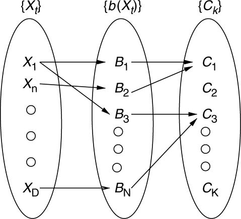
While each mapped location is assigned to a single cluster, each cluster consists of multiple (at least two) mapped locations. Each matepair can have a number of potential mapped locations. In other words, the set of matepairs and mapped locations have a one-to-many relationship, while each mapped location is a member of at most one cluster. This is illustrated in Figure 6.
Fig. 6.
This diagram illustrates the relationship between the set of matepairs, {Xt}, mapped locations {b(Xt)}, and clusters {Ck} after the clustering phase. The goal of our algorithm is to find an assignment of each matepair to a single mapped location, and hence to a single cluster.
We assume that each matepair is involved in at most one structural variation, hence there should be a many-to-one correspondence between the set of matepairs and the set of clusters. To map each matepair to a unique cluster, we search for a valid configuration, ω, that has a one-to-one mapping between {Xt} and {b(Xt)}. Furthermore, we wish to find the configuration that maximizes the objective function J(ω).
The objective function J(ω) is defined as follows:
Here, λi is a weight parameter for each feature fi, trained as described below in Section 2.4.3.
The three features used in our framework are sequence similarity (the percent identity of the alignment between the read and the reference genome), the probability that the cluster is genuine given the matepairs, and the number of matepairs mapped to the cluster.
The sequence similarity feature is
where z(b(Xt)) is the percent identity of the mapping b(Xt) and K is the number of clusters.
The second feature is the product of probabilities that cluster Ck is a genuine cluster given the matepairs which are assigned to Ck. Larger probabilities imply that the cluster Ck is reliable. This is defined as follows:
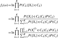 |
where L is the number of matepairs involved in cluster Ck, and  is the lth matepair involved in Ck. Here, we assume that {Xt} provide independent support for the cluster. To compute
  , we use the average of log conditional probabilities of matepairs
  as follows:
where Ck is a cluster consisting of  and Xj∈Ck. This approximation allows us to reuse the implementation for computing linkages in Section 2.4.1.
We define the prior probability of P(Ck) as follows:
 |
The final feature is related to the cardinality of the clusters. Intuitively, we assume that clusters having a large number of matepairs are more reliable than ones with a smaller number. Thus, when deciding the cluster to which to assign a particular matepair, we want to choose the mapped location b(Xt) which belongs to the cluster Ck, such that |Ck|≥|Cj| for all Cj, where j≠k. Thus, the definition of the third feature is
2.4.3 Parameter learning
We have three parameters, λ1, λ2 and λ3 in the objective function J. To train these, we use the softmax regression/maximum entropy model (Della Pietra et al., 1997). Let Ω be the set of all valid configurations (where each matepair is assigned to a single cluster). We define a distribution over the configurations ω∈Ω:
where Z is the partition function and ∑iλi is a fixed constant.
We rescale the three features f1(ω), f2(ω), f3(ω) so that for each feature, the highest observed value is one, and the lowest is zero, prior to running the hill climbing procedure.
Given a sampling of the configurations after the clustering phase, we learn parameters by maximizing the log likelihood
where θ={λ1, λ2, λ3} is the set of parameters. We use a hill climbing search to locally maximize L(θ).
While initially we set all λi=1, the hill climbing search yielded weights 0.10, 0.14 and 2.76 for the three features: sequence similarity, cluster probability, and cardinality respectively.
2.4.4 Local search to optimize J(ω)
Before maximizing the objective function J using a hill climbing algorithm, we initialize the configuration with a greedy method so that the local search starts from a good location. We use the following algorithm:
1. Determine the set of clusters identified by the clustering algorithm of Section 2.4.1.
2. Sort all matepairs based on the number of mapped locations.
3. For all matepairs Xt starting with those with the fewest mapped locations, assign each to the cluster Ck that locally maximizes the objective function J.
After the initial assignment, we perform a local hill climbing search to optimize J(ω). At each step of the algorithm, we find a matepair Xt that we can move from its current cluster to another one, while increasing the objective function. As soon as no such move exists, our algorithm terminates.
3 EXPERIMENTAL RESULTS
3.1 Dataset and parameters
We have downloaded the repeat-masked NCBI version hg18 of the human genome (Lander et al., 2001) from the UCSC Genome Browser (Kent et al., 2002), and the matepairs corresponding to the recently published diploid human genome (referred to as the JCVI donor) (Levy et al., 2007) from the NCBI Trace Archive (http://www.ncbi.nlm.nih.gov/Traces/).1
All reads were quality trimmed to the longest span with at most 10 low quality (Q≤20) residues in any window of 40 residues. Any read with length ≤200 after the trimming process was discarded. The remaining reads were mapped to the reference genome using BLAT (Kent, 2002) with the -mask=lower option. We also removed all BLAT hits with less than 150 bases outside of any repeat annotated by RepeatMasker (as downloaded from the UCSC Browser). For every read we considered matches to the genome at ≥95% identity, selecting up to the top 20 matches. We computed the probability distribution p(Y) for every insert size (from 1925 bp to 45 kb) as described above.
For all matepairs, if any pair of BLAT hits for its two reads were concordant with the insert size (mapped at a distance <2σ from the mean), the clone was considered to be supported by the genome, and was discarded from clustering analysis.
Table 1 summarizes the resulting data. The majority of the matepairs had concordant hits (94%) and mapped to unique locations in the genome (93%). The remaining reads varied widely in the number of mapped locations (we only considered the top 400 mapped locations based on the sequence similarity for each matepair).
Table 1.
The rows correspond to M=α · β, the number of mapped locations for the matepairs in the group. The overall column shows the total percentage of all matepairs in each category. The concordant column shows the percentage of matepairs having a pair of BLAT hits with a mapped location deviating <2σ from the mean insert size, and the discordant are the remainder
| Type | Overall | Concordant | Discordant |
|---|---|---|---|
| 1 | 92.8 | 96.1 | 3.9 |
| 2–5 | 2.7 | 83.7 | 16.3 |
| 6–10 | 0.9 | 77.2 | 22.8 |
| 11–20 | 0.7 | 70.1 | 29.9 |
| 21–100 | 2.4 | 38.4 | 61.6 |
| 101–400 | 0.3 | 68.6 | 31.4 |
We used these data to generate a set of clusters, as described in the Methods sections. We further filtered the putative insertions and deletions by computing the P-values of all clusters and considering only the most confident, allowing for a false discovery rate (Benjamini and Hochberg, 1995) of 5%. Because translocations are biologically less likely, we further filtered out any predicted translocation if the cluster suggesting it did not have at least one matepair mapped only to that location.
In the next two sections we analyze the results of our clusterings, first by comparing our insertion, deletion, and inversion predictions to three previously described datasets of structural variants, and then by analyzing the inter-chromosomal events located by our method.
3.2 Analysis of insertions, deletions and inversions
Our algorithm predicted 1578 insertions, 2615 deletions, and 373 inversions between the reference NCBI human genome and the JCVI donor. Of these, 1374, 2279 and 185, respectively, were supported by at least a single uniquely mapped matepair. 199 inversion variants were double-ended (had a cluster at both inversion endpoints). The disparity in the number of insertions and deletions discovered by our algorithm is due to two causes. The first is that via the clone-end mapping strategy it is impossible to locate insertions which are longer than the clone size. As the bulk of the clones used to sequence the JCVI donor were ≈10 kb in length, many of the larger insertions could not be discovered. Another potential bias originates in the assembly of the reference human genome, which is more likely to use a longer allele within a heterozygous locus. In this section we compare our results to the Tuzun, Korbel and Levy datasets (for the last dataset, we only consider variants found using sequence comparisons) curated at the Database of Genomic Variants (DGV), as well as to the whole DGV database. The results are summarized in Table 2.
Table 2.
A comparison of the structural variants located by our approach with the datasets generated by Tuzun et al., (2005) Levy et al., (2007), Korbel et al., (2007), and all insertion, deletion, and inversion variants in the DGV database (Iafrate et al., 2004). The Variants row indicates the total number of events of each type identified by our algorithm, while the rows for each study show the Total number of rearrangements of this type found by the study as well as the number of variants that overlap Any variant from our dataset, our variants with a Unique matepair, and a homozygous (Hom) event, respectively. For inversion we separately note the events where both ends were detected (double-ended inversions, Dbl)
| Type | Insertion |
Deletion |
Inversion |
||||||||||
|---|---|---|---|---|---|---|---|---|---|---|---|---|---|
| Total | Any | Unique | Hom | Total | Any | Unique | Hom | Total | Any | Dbl | Unique | Hom | |
| Variations | 1578 | NA | 1374 | 50 | 2615 | NA | 2279 | 81 | 373 | NA | 199 | 185 | 7 |
| Tuzun | 139 | 39 | 34 | 5 | 102 | 54 | 47 | 9 | 56 | 46 | 40 | 41 | 4 |
| Levy | 319 | 94 | 91 | 20 | 344 | 181 | 172 | 39 | NA | NA | NA | NA | NA |
| Korbel | 34 | 0 | 0 | 0 | 742 | 321 | 296 | 48 | 105 | 71 | 67 | 69 | 6 |
| DGV-All | 2216 | 163 | 116 | 10 | 4697 | 1117 | 1000 | 124 | 164 | 118 | 108 | 111 | 11 |
Our predicted set of structural variants shows a clear correlation with the results of the previous studies. Anywhere between 41% (inversions) and 14% (insertions) of the events located by our algorithm overlap an already known event. While our results show a large overlap with all three of the datasets, we also predict a much larger number of structural variants, as we are working with a larger input set of matepairs. We computed a P-value for the correlation between our results and all of the datasets described in Table 2, and found these to be significantly correlated (P<0.001 based on Monte Carlo simulations).
Perhaps more surprising than the similarity between our results and the previously described structural variants are the differences: we identify 3464 insertion, deletion, and inversion structural variants that do not overlap any structural variant in the DGV (Iafrate et al., 2004), of which 3032 have support from a uniquely mapped matepair.
In (Levy et al., 2007), the 20 largest insertions and 20 largest deletions identified in the JCVI donor were validated by fosmid-end mapping. The authors were able to validate all 20 insertions and 17/20 deletions. Our set of putative variants contains 13 of the 20 validated insertion variants, as well as all 17 of the 17 deletion variants. Of the seven insertion variants not predicted by our approach, four were larger than the largest insert size, and hence could not be found by clone-end mapping. For the other three insertions we found no discordant matepairs in the proximity of the variants. Notably, all of the three deletions that could not be validated in (Levy et al., 2007) were absent from our predictions.
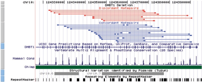
An example of an indel found by our algorithm that had been validated through fosmid end-mapping from unrelated individuals is a deletion in the DMBT1 (Deleted in Malignant Brain Tumor 1) gene located on chromosome 10q26. The cluster supporting this 12 kilobase deletion consists of 9 matepairs and had a P-value of 1.75 × 10⁻¹³. The deletion location is localized to within 6 kb (Figure 7) and contains 10 of the 40 exons of the DMBT1 gene. This deletion overlaps a known deletion from the Tuzun dataset, and was identified in Levy et al.'s analysis as homozygous in the Venter genome. However, our analysis indicated an approximately equal number of concordant and discordant matepairs in the cluster. Additionally the authors of the original JCVI study have noticed a 2-fold decrease in the coverage at this locus, and a high number of reads whose pairs are located on a different scaffold (Samuel Levy, personal communication). This suggests that this is likely a heterozygous, rather than a homozygous deletion. Furthermore, the conservation between the human reference genome and the chimpanzee genome at the locus suggests that the allele without the deletion is ancestral.
Fig. 7.
A display of the DMBT1 gene from the UCSC Genome Browser with a custom track showing the mapped locations of the three matepairs supporting a deletion in the JCVI donor's genome. The nine discordant matepairs (top of the figure) are supporting a deletion of size ≈ 12 Kb. The 18 concordant matepairs mapping to both the left and right sides of the cluster demonstrate that the variant is heterozygous. Furthermore the continuous alignment with the chimpanzee genome indicates that the ancestral allele is likely the one without the deletion.
3.3 Analysis of translocation variants
Our algorithm, unlike the previous approaches of Tuzun and Korbel, characterizes not only insertions, deletions, and inversions, but also translocation variants. Translocations are extremely rare events, hence it is quite likely that many of the events that we are labeling as ‘translocations’—those characterized by the two ends of a clone being mapped on different chromosomes—are in reality combinations of simpler events (e.g. a duplication followed by a deletion). Due to the low likelihood of such an event (or series of events), we only predicted a translocation polymorphism when: 1) there was at least one matepair for which the translocation mapping was unique, and 2) for all of the other matepairs, there were no mapped locations that had both ends of the clone on the same chromosome.
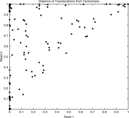
It is known that the centromeres are ‘hot-spots’ for rearrangements, including translocations, jumping translocations, and duplications, (Berger and Bernard, 2007; Jackson et al., 1999; Rudd and Willard, 2004; She et al., 2004). We classified each translocation's two endpoints based on their distance from the centromere, normalized between zero and one. The results are summarized in Figure 8. As expected, of the 163 translocation variants, a significant fraction (59%) had at least one endpoint within 4.5 Mb from the centromeres.
Fig. 8.
The scatter plot illustrating the locations of the 163 translocation variants relative to the centromeres: 0 is the centromere, 1 is the telomere. The plot illustrates that most translocations have one of their ends near a centromere, and the other proximal to either the centromere or a telomere.
While some fraction of these results may be due to incorrect mapping of reads, we believe this is not likely, as we require that none of the matepairs have any pair of mapped locations on the same chromosomes. It is possible that some fraction of these can be explained biologically. However, another explanation for these events are errors in the reference human genome assembly, as the centromeres are known to be difficult to assemble due to a large number of repetitive sequences.
4 DISCUSSION
In this study, we propose a probabilistic framework for identify-ing structural variations. Our method, while sharing the overall vadjust clone-end mapping strategy introduced by Tuzun et al.), and employed by Korbel et al., (2007) and Tuzun et al., (2005), differs significantly in that we do not assign the best mapped location to every mate pair, but rather search over the space of all possible assignments in order to optimize our overall confidence in all of the variations identified. Unlike the previous approaches, we make use of not only discordant matepairs, but also concordant ones in order to determine if a variant is homozygous and to compute P-values for insertion and deletion events. One promising avenue for further improvement is the use of concordant matepairs to identify false-positive clusters: if only a few discordant matepairs support a cluster, while many concordant ones contradict it, the cluster is likely to be a false positive.
The problem of detecting structural variations from matepair data contains many significant challenges. For example, one limitation of our approach is that it ignores microarray data that predict the copy number variations (CNVs) present in the JCVI donor's genome. The development of methods that combine information from various sources in order to better predict and classify the variations is an important avenue for future work.
ACKNOWLEDGEMENTS
We are grateful to Alexey Kondrashov, Lars Feuk, Stephen Scherer, Yevgeny Brudno and Andy Pang for useful discussions, Paul Medvedev and Stephen Rumble for a critical reading of the manuscript, and the anonymous reviewers.
Funding: This research was funded by an NSERC Discovery Grant, Canada Foundation for Innovation, and NIH R01 grant GM81080-01.
Conflict of Interest: none declared.
Footnotes
1Downloaded Dec. 10, 2007, query: center_name=‘JCVI’ and species _code=‘HOMO SAPIENS’ and center_project‘GENOMIC-SEQUENCING-DIPLOID-HUMAN-REFERENCE-GENOME’ and strategy=‘WGA’ and trace_code_type=‘WGS’
REFERENCES
- Benjamini Y, Hochberg Y. Controlling the false discovery rate: a practical and powerful approach to multiple testing. Journal of the Royal Statistical Society. Series B (Methodological) 1995;57:289–300. [Google Scholar]
- Berger R, Bernard OA. Jumping translocations. Genes, Chromosomes and Cancer. 2007;46:717. doi: 10.1002/gcc.20456. [DOI] [PubMed] [Google Scholar]
- Della Pietra S, et al. Inducing features of random fields. IEEE Transactions on Pattern Analysis and Machine Intelligence. 1997;19:380–393. [Google Scholar]
- Feuk L, et al. Structural variation in the human genome. Nat. Rev. Genet. 2006;7:85–97. doi: 10.1038/nrg1767. [DOI] [PubMed] [Google Scholar]
- Fowlkes EB, Mallows CL. A Method for Comparing TwoHierarchical Clusterings. Journal of the American Statistical Association. 1983;78:553–569. [Google Scholar]
- Iafrate AJ, et al. Detection of large-scale variation in the human genome. Nature Genetics. 2004;36:949–951. doi: 10.1038/ng1416. [DOI] [PubMed] [Google Scholar]
- Jackson MS, et al. Sequences flanking the centromere of human chromosome 10 are a complex patchwork of arm-specific sequences, stable duplications and unstable sequences with homologies to telomeric and other centromeric locations. Human Molecular Genetics. 1999;8:205–215. doi: 10.1093/hmg/8.2.205. [DOI] [PubMed] [Google Scholar]
- Kallioniemi A, et al. Comparative genomic hybridization for molecular cytogenetic analysis of solid tumors. Science. 1992;258:818–821. doi: 10.1126/science.1359641. [DOI] [PubMed] [Google Scholar]
- Kent WJ. BLAT—The BLAST-Like Alignment Tool. Genome Research. 2002;12:996–1006. doi: 10.1101/gr.229202. [DOI] [PMC free article] [PubMed] [Google Scholar]
- Kent WJ, et al. The Human Genome Browser at UCSC. Genome Research. 2002;12:656–664. doi: 10.1101/gr.229102. [DOI] [PMC free article] [PubMed] [Google Scholar]
- Korbel JO, et al. Paired-end mapping reveals extensive structural variation in the human genome. Science. 2007;318:420. doi: 10.1126/science.1149504. [DOI] [PMC free article] [PubMed] [Google Scholar]
- Lander ES, et al. Initial sequencing and analysis of the human genome. Nature. 2001;409:860–921. doi: 10.1038/35057062. [DOI] [PubMed] [Google Scholar]
- Levy S, et al. The diploid genome sequence of an individual human. PLoS Biol. 2007;5:e254. doi: 10.1371/journal.pbio.0050254. [DOI] [PMC free article] [PubMed] [Google Scholar]
- Lucito R, et al. Representational Oligonucleotide Microarray Analysis: a High-Resolution Method to Detect Genome Copy Number Variation. Genome Research. 2003;13:2291–2305. doi: 10.1101/gr.1349003. [DOI] [PMC free article] [PubMed] [Google Scholar]
- Mills RE, et al. An initial map of insertion and deletion (INDEL) variation in the human genome. Genome Research. 2006;16:1182. doi: 10.1101/gr.4565806. [DOI] [PMC free article] [PubMed] [Google Scholar]
- Rudd MK, Willard HF. Analysis of the centromeric regions of the human genome assembly. Trends in Genetics. 2004;20:529–533. doi: 10.1016/j.tig.2004.08.008. [DOI] [PubMed] [Google Scholar]
- She X, et al. The structure and evolution of centromeric transition regions within the human genome. Nature. 2004;430:857–864. doi: 10.1038/nature02806. [DOI] [PubMed] [Google Scholar]
- The International HapMap Consortium. The International HapMap Project. Nature. 2003;426:789–796. doi: 10.1038/nature02168. [DOI] [PubMed] [Google Scholar]
- Tuzun E, et al. Fine-scale structural variation of the human genome. Nature Genetics. 2005;37:727–732. doi: 10.1038/ng1562. [DOI] [PubMed] [Google Scholar]


